Galton and Regression toward the Mean

GALTON AND REGRESSION TOWARD THE MEAN

Francis Galton (1822–1911), an anthropologist and adherent of the scientific beliefs of his cousin Charles Darwin, studied the heritability of such human characteristics as physical traits (height and weight) and mental attributes (personality dimensions and mental capabilities). Believing that human characteristics could be inherited, he was a supporter of the eugenics movement, which sought to improve human beings through selective mating.

Given his interest in how human traits are passed from one generation to the next, he embarked in 1884 on a testing program at the South Kensington Museum in London, England. At his laboratory in the museum, he collected data from fa-thers and sons on a range of physical and sensory characteristics. He observed among his study group that characteristics such as height and weight tended to be inherited. However, when he examined the children of extremely tall parents and those of extremely short parents, he found that although the children were tall or short, they were closer to the population average than were their parents. Fathers who were taller than the average father tended to have sons who were taller than av-erage. However, the average height of these taller than average sons tended to be lower than the average height of their fathers. Also, shorter than average fathers tended to have shorter than average sons; but these sons tended to be taller on aver-age than their fathers.

Galton also conducted experiments to investigate the size of sweet pea plants produced by small and large pea seeds and observed the same phenomenon for a successive generation to be closer to the average than was the previous generation. This finding replicated the conclusion that he had reached in his studies of humans.

Galton coined the term “regression,” which refers to returning toward the aver-age. The term “linear regression” got its name because of Galton’s discovery of this phenomenon of regression toward the mean. For more specific information on this topic, see Draper and Smith (1998), page 45.

Returning to the relationship that Galton discovered between the height at adult-hood of a father and his son, we will examine more closely the phenomenon of re-gression toward the mean. Galton was one of the first investigators to create a scat-ter plot in which on one axis he plotted heights of fathers and on the other, heights of sons. Each single data point consisted of height measurements of one father–son pair. There was clearly a high positive correlation between the heights of fathers and the heights of their sons. He soon realized that this association was a mathemat-ical consequence of correlation between the variables rather than a consequence of heredity.

The paper in which Galton discussed his findings was entitled “Regression to-ward mediocrity in hereditary stature.” His general observations were as follows: Galton estimated a child’s height as

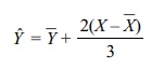
 where Yˆ is the predicted or estimated child’s height, Yˆ is the average height of the children, X is the parent’s height for that child, and  is the average height of all parents. Apparently, the choice of X was a weighted average of the mother’s and father’s heights.

From the equation you can see that if the parent has a height above the mean for parents, the child also is expected to have a greater than average height among the children, but the increase Yˆ =  is only 2/3 of the predicted increase of the parent over the average for the parents. However, the interpretation that the children’s heights tend to move toward mediocrity (i.e., the average) over time is a fallacy sometimes referred to as the regression fallacy.

In terms of the bivariate normal distribution, if Y represents the son’s height and X the parent’s height, and the joint distribution has mean μ_x for X, mean μ_y for Y, standard deviation σ_x for X, standard deviation σ_y for Y, and correlation ρ_xy between X and Y, then E(Y – μ_y|X = x) = ρ_xy σ_y (x – μ_x)/σ_x.

If we assume σ_x = σ_y, the equation simplifies to ρ_xy(x – μ_x). The simplified equa-tion shows mathematically how the phenomenon of regression occurs, since 0 < ρ_xy < 1. All of the deviations of X about the mean must be reduced by the multiplier ρ_xy, which is usually less than 1. But the interpretation of a progression toward mediocrity is incorrect. We see that our interpretation is correct if we switch the roles of X and Y and ask what is the expected value of the parent’s height (X) given the son’s height (Y), we find mathematically that E(X – μ_x|Y = y) = ρ_xy σ_x(y – μ_y)/σ_y, where μ_y is the overall mean for the population of the sons. In the case when σ_x = σ_y, the equation simplifies to ρ_xy(y – μ_y). So when y is greater than μ_y, the expected value of X moves closer to its overall mean (μ_x) than Y does to its overall mean (μ_y).

Therefore, on the one hand we are saying that tall sons tend to be shorter than their tall fathers, whereas on the other hand we say that tall fathers tend to be short-er than their tall sons. The prediction for heights of sons based on heights of fathers indicates a progression toward mediocrity; the prediction of heights of fathers based on heights of sons indicates a progression away from mediocrity. The fallacy lies in the interpretation of a progression. The sons of tall fathers appear to be shorter be-cause we are looking at (or conditioning on) only the tall fathers. On the other hand, when we look at the fathers of tall sons we are looking at a different group because we are conditioning on the tall sons. Some short fathers will have tall sons and some tall fathers will have short sons. So we err when we equate these conditioning sets. The mathematics is correct but our thinking is wrong. We will revisit this fallacy again with students’ math scores.

When trends in the actual heights of populations are followed over several gen-erations, it appears that average height is increasing over time. Implicit in the re-gression model is the contradictory conclusion that the average height of the popu-lation should remain stable over time. Despite the predictions of the regression model, we still observe the regression toward the mean phenomenon with each gen-eration of fathers and sons.

Here is one more illustration to reinforce the idea that interchanging the predic-tor and outcome variables may result in different conclusions. Michael Chernick’s son Nicholas is in the math enrichment program at Churchville Elementary School in Churchville, Pennsylvania. The class consists of fifth and sixth graders, who take a challenging test called the Math Olympiad test. The test consists of five problems, with one point given for each correct answer and no partial credit given. The possi-ble scores on any exam are 0, 1, 2, 3, 4, and 5. In order to track students’ progress, teachers administer the exam several times during the school year. As a project for the American Statistical Association poster competition, Chernick decided to look at the regression toward the mean phenomenon when comparing the scores on one exam with the scores on the next exam.

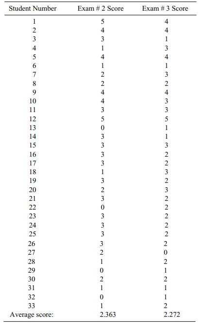
Chernick chose to compare 33 students who took both the second and third ex-ams. Although the data are not normally distributed and are very discrete, the linear model provides an acceptable approximation; using these data, we can demonstrate the regression toward the mean phenomenon. Table 12.7 shows the individual stu-dent’s scores and the average scores for the sample for each test.

Figure 12.10 shows a scatter plot of the data along with the fitted least squares regression line, its equation, and the square of the correlation.

The term R² (Pearson correlation coefficient squared) when multiplied by 100 refers to the percentage of variance that an independent variable (X) accounts for in the dependent variable (Y). To find the Pearson correlation coefficient estimate of the relationship between scores for exam # 2 and exam # 3, we need to find the square root of R², which is shown in the figure as 0.3901; thus, the Pearson correla-tion coefficient is 0.6246. Of the total variance in the scores, almost 40% of the variance in the exam # 3 score is explained by the exam # 2 score. The variance in exam scores is probably attributable to individual differences among students. The average scores for exam # 2 and exam # 3 are 2.363 and 2.272, respectively (refer to Table 12.7).

TABLE 12.7. Math Olympiad Scores

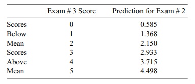
In Table 12.8, we use the regression equation shown in Figure 12.10 to predict the individual exam # 3 scores based on the exam # 2 scores. We also can observe the regression toward the mean phenomenon by noting that for scores of 0, 1, and 2 (all below the average of 2.272 for exam # 3), the predicted values for Y are higher than the actual scores, but for scores of 3, 4, and 5 (all above the mean of 2.272), the predicted values for Y are lower than the actual scores. Hence, all predicted scores (Yˆs) for exam # 3 are closer to the overall class mean for exam # 3 than are the actual exam # 2 scores.

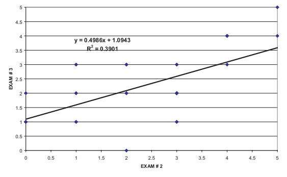
Figure 12.10. Linear regression of olympiad scores of advanced students predicting exam # 3 from exam # 2.

Note that a property of the least squares estimate is that if we use x = 2.363, the mean for the x’s, then we get an estimate of y = 2.272, the mean of the y’s. So if a student had a score that was exactly equal to the mean for exam # 2, we would pre-dict that the mean of the exam # 3 scores would be that student’s score for exam # 3. Of course, this hypothetical example cannot happen because the actual scores can be only integers between 0 and 5.

Although the average scores on exam # 3 are slightly lower than the average scores on exam # 2. the difference between them is not statistically significant, according to a paired t test (t = 0.463, df = 32).

TABLE 12.8. Regression toward the Mean Based on Predicting Exam #3 Scores from Exam # 2 Scores

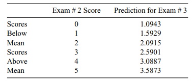
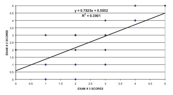
Figure 12.11. Linear regression of olympiad scores predicting exam # 2 from exam # 3, advanced stu-dents (tests reversed).

To demonstrate that it is flawed thinking to surmise that the exam # 3 scores tend to become more mediocre than the exam # 2 scores, we can turn the regression around and use the exam # 3 scores to predict the exam # 2 scores. Figure 12.11 ex-hibits this reversed prediction equation.

Of course, we see that the R² value remains the same (and also the Pearson cor-relation coefficient); however, we obtain a new regression line from which we can demonstrate the regression toward the mean phenomenon displayed in Table 12.9.

Since the average score on exam # 2 is 2.363, the scores 0, 1, and 2 are again be-low the class mean for exam # 2 and the scores 3, 4, and 5 are above the class mean for exam # 2. Among students who have exam # 3 scores below the mean, the pre-diction is for their scores on exam # 2 to increase toward the mean score for exam #2. The corresponding prediction among students who have exam # 3 scores above the mean is that their scores on exam # 2 will decrease. In this case, the degree of shift between actual and predicted scores is less than in the previous case in which exam # 2 scores were used to predict exam # 3 scores. Again, according to an im-portant property of least squares estimates, if we use the exam # 3 mean of 2.272 for x, we will obtain the exam # 2 mean of 2.363 for y (which is exactly the same value for the mean of exam # 2 shown in Table 12.7)

TABLE 12.9. Regression toward the Mean Based on Predicting Exam # 2 Scores from Exam # 3 Scores

Now let’s examine the fallacy of our thinking regarding the trend in exam scores toward mediocrity. The predicted scores for exam # 3 are closer to the mean score for exam # 3 than are the actual scores on exam # 2. We thought that both the lower predicted and observed scores on exam # 3 meant a trend toward mediocrity. But the predicted scores for exam # 2 based on scores on exam # 3 are also closer to the mean of the actual scores on exam # 2 than are the actual scores on exam # 3. This finding indicates a trend away from mediocrity in moving in time from scores on exam # 2 to scores on exam # 3. But this is a contradiction because we observed the opposite of what we thought we would find. The flaw in our thinking that led to this contradiction is the mistaken belief that the regression toward the mean phenome-non implies a trend over time.

The fifth and sixth grade students were able to understand that the better students tended to receive the higher grades and the weaker students the lower grades. But chance also could play a role in a student’s performance on a particular test. So stu-dents who received a 5 on an exam were probably smarter than the other students and also should be expected to do well on the next exam. However, because the maximum possible score was 5, by chance some students who scored 5 on one exam might receive a score of 4 or lower on the next exam, thus lowering the ex-pected score below 5.

Similarly, a student who earns a score of 0 on a particular exam is probably one of the weaker students. As it is impossible to earn a score of less than 0, a student who scores 0 on the first exam has a chance of earning a score of 1 or higher on the next exam, raising the expected score above 0. So the regression to the mean phe-nomenon is real, but it does not mean that the class as a group is changing. In fact, the class average could stay the same and the regression toward the mean phenome-non could still be seen.