Kruskal–Wallis Test: One-Way ANOVA by Ranks
| Home | | Advanced Mathematics |Chapter: Biostatistics for the Health Sciences: Nonparametric Methods
To describe the test procedure, we need to use some mathematical notation. Let Xij represent the jth observation from the ith population. We assume that there are k ≥ 3 populations and for population i we have ni observations.
KRUSKAL–WALLIS TEST: ONE-WAY ANOVA BY RANKS
The Kruskal–Wallis test is a nonparametric analog
to the one-way analysis of variance discussed in Chapter 13. It is a simple
generalization of the Wilcoxon rank-sum test. The problem is to identify
whether or not three or more populations (inde-pendent samples) have the same
distribution (or central tendency). We test the null hypothesis (H0) that the distributions of
the parent populations are the same against the alternative (H1) that the distributions
are different. The rationale for the test in-volves pooling all of the data and
then applying a rank transformation. If the null hypothesis is true, each group
should have rank sums that are similar. If at least one group has a higher (or
lower) median than the others, it should have a higher (or lower) rank sum.
Table 14.8 provides an example of data layout for several samples (e.g., k samples), following the model for the
Kruskal–Wallis test.
To describe the test procedure, we need to use some mathematical notation. Let Xij represent the jth observation from the ith population. We assume that there are k ≥ 3 populations and for population i we have ni observations.
TABLE 14.8. Data Layout for Kruskal–Wallis Test
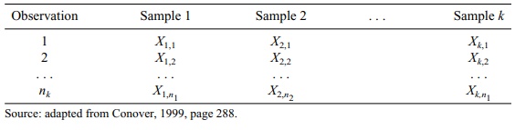
N = the total number of observations. Let N = Σik=1ni and for each i let Ri be the sum of the ranks for the observations in the ith population. That is, Ri = Σjn=1iR(Xij)
for each i, where i = 1, 2, . . . , k). The test statistic is defined as
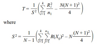
In the absence of ties, S2 simplifies to N(N + 1)/12, and T is defined by the following equation for a chi-square
approximation to the Kruskal–Wallis rank test for comparing three or more
independent samples (no ties) is
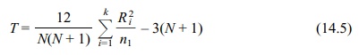
where ni
is the sample size for the ith
population and N is the total sample
size.
This test statistic has a distribution with a
chi-square approximation when there are no ties. Under the null hypothesis that
the distributions are the same, the test sta-tistic’s distribution has been
tabulated for small values of N. The
tables of critical values for T are
not included in this text. When N is
large, an approximate chi-square distribution can be used. In fact, the test
statistic T has approximately a
chi-square distribution with k – 1
degrees of freedom, where k again
refers to the number of samples. The approximate test has been shown to work
well even when N is not very large.
See Conover (1999) for details and references.
Equation 14.6 gives the chi-square approximation to
the Kruskal–Wallis rank test for comparing three or more independent samples in
the event of ties:
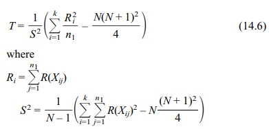
ni is the sample size for the ith population
N is the total sample size
The SAS procedure NPAR1WAY can be used to perform
the Kruskal–Wallis test. That procedure also allows you to compare the results
to the F test used for a one-way
ANOVA.
To illustrate the Kruskal–Wallis test, we take an
example from Conover (1999). In this example, three instructors are compared to
determine whether they are simi-lar or different in their grading practices.
(See Table 14.9.). This example demon-strates a special case in which there are
many ties, which occur because the ordinal data have a restricted range.
Table 14.9 provides the rankings for these data. As
is usual with grades, f is the lowest
rank, then D, then C, then B, and finally A. From the pooled total we see that
the number of Fs given by the three instructors is 9. As a result, each of the
9 students gets an average rank of 5 = (9 + 1)/2. The respective counts and
rank-ings for the remaining grades are D
(19, rank 19), C (34, rank 46.5), B
(27, rank 76), and A (20, rank 99.5). The ranking of 19 for Ds is based on the
fact that there are 9 Fs and 19 Ds. So the rank for Ds is 9 + (19 + 1)/2 = 9 +
10 = 19. The rank for Cs comes from 28 Ds and Fs along with 34 Cs for 28 + (34
+ 1)/2 = 28 + 17.5 = 45.5. For Bs we get the rank from 62 Cs, Ds and Fs along
with 27 Bs for 62 + (27 + 1)/2 = 62 + 14 = 76. Finally, the rank for the As is
obtained by taking the 89 Bs, Cs, Ds and Fs along with 20 As for 89 + (20 +
1)/2 = 89 + 10.5 = 99.5. Conover (1999) chooses to rank the As with the lowest
rank and the Fs with the highest rank. We chose to give As the highest rank and
Fs the lowest. For pur-poses of the analysis, assigning the highest rank to A
or f does not affect the out-come of
the test. Our choice was made because we like to think of high ranks
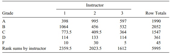
cor-responding to high grades. For each cell in Table 14.9, we multiply the
number shown in the cell by the rank for that row (e.g., 4 × 99.5 = 398. Table
14.10 shows the resulting values; for example, the value in cell one is 398.
Then we ap-ply the formulas in Equation 14.6. Based on the formula for S2, we see that S2 = {(5)2 9 +
(19)2 19 + (45.5)2 34 + (76)2 27 + (99.5)2
20 –109 (110)2/4}/108 = 941.708 and T = {(2359.5)2/43 + (2023.5)2/38 + (1612)2/28–109(110)2/4}/S2 = 0.321. These results for
T and S2 are identical to Conover’s, even though we ranked the
grades in the opposite way. Based on the approximate chi-square with 2 degrees
of freedom distribution for T, the critical value for α = 0.05 is 5.991. Because our
calculated T = 0.321, the association
between instructors and grades assigned is not statistically significant.
TABLE 14.9. Grade Counts for Students by Instructor
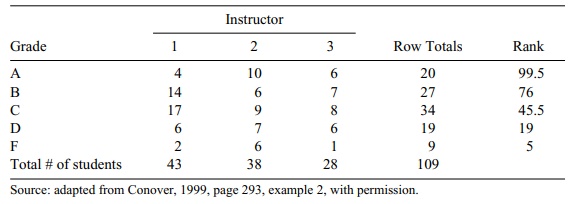
TABLE 14.10. Ranks for Grade Counts for Students by Instructor
Related Topics
