Measures of Dispersion

MEASURES OF DISPERSION

As you may have observed already, when we select a sample and collect measurements for one or more characteristics, these measurements tend to be different from one another. To give a simple example, height measurements taken from a sample of persons obviously will not be all identical. In fact, if we were to take measure-ments from a single individual at different times during the day and compare them, the measurements also would tend to be slightly different from one another; i.e., we are shorter at the end of the day than when we wake up!

How do we account for differences in biological and human characteristics? While driving through Midwestern cornfields when stationed in Michigan as a post-doctoral fellow, one of the authors (Robert Friis) observed that fields of corn stalks generally resemble a smooth green carpet, yet individual plants are taller or shorter than others. Similarly, in Southern California where oranges are grown or in the al-mond orchards of Tuscany, individual trees differ in height. To describe these dif-ferences in height or other biological characteristics, statisticians use the term vari-ability.

We may group the sources of variability according to three main categories: true biological, temporal, and measurement. We will delimit our discussion of the first of the categories, variation in biological characteristics, to human beings. A range of factors cause variations in human biological characteristics, including, but not limited to, age, sex, race, genetic factors, diet and lifestyle, socioeconomic status, and past medical history.

There are many good examples of how each of the foregoing factors produces variability in human characteristics. However, let us focus on one—age, which is an important control or demographic variable in many statistical analyses. Biological characteristics tend to wax and wane with increasing age. For example, in the U.S., Europe, and other developed areas, systolic and diastolic blood pressures tend to in-crease with age. At the same time, age may be associated with decline in other char-acteristics such as immune status, bone density, and cardiac and pulmonary func-tioning. All of these age-related changes produce differences in measurements of characteristics of persons who differ in age. Another important example is the im-pact of age or maturation effects on children’s performance on achievement tests and intelligence tests. Maturation effects need to be taken into account with respect to performance on these kinds of tests as children progress from lower to higher levels of education.

Temporal variation refers to changes that are time-related. Factors that are capa-ble of producing temporal variation include current emotional state, activity level, climate and temperature, and circadian rhythm (the body’s internal clock). To illus-trate, we are all aware of the phenomenon of jet lag—how we feel when our normal sleep–awake rhythm is disrupted by a long flight to a distant time zone. As a conse-quence of jet lag, not only may our level of consciousness be impacted, but also physical parameters such as blood pressure and stress-related hormones may fluctu-ate. When we are forced into a cramped seat during an extended intercontinental flight, our circulatory system may produce life-threatening clots that lead to pulmonary embolism. Consequently, temporal factors may cause slight or sometimes major variations in hematologic status.

Finally, another example of a factor that induces variability in measurements is measurement error. Discrepancies between the “true” value of a variable and its measured value are called measurement errors. The topic of measurement error is an important aspect of statistics. We will deal with this type of error when we cover regression (Chapter 12) and analysis of variance (Chapter 13). Sources of measure-ment error include observer error, differences in measuring instruments, technical errors, variability in laboratory conditions, and even instability of chemical reagents used in experiments. Take the example of blood pressure measurement: In a multi-center clinical trial, should one or more centers use a faulty sphygmomanometer, that center would contribute measures that over- or underestimate blood pressure. Another source of error would be inaccurate measurements caused by medical per-sonnel who have hearing loss and are unable to detect blood pressure sounds by lis-tening with a stethoscope.

Several measures have been developed—measures of dispersion—to describe the variability of measurements in a data set. For the purposes of this text, these measures include the range, the mean absolute deviation, and the standard deviation. Percentiles and quartiles are other measures, which we will discuss in Chapter 6.

1. Range

The range is defined as the difference between the highest and lowest value in a dis-tribution of numbers. In order to compute the range, we must first locate the highest and lowest values. With a small number of values, one is able to inspect the set of numbers in order to identify these values.

When the set of numbers is large, however, a simple way to locate these values is to sort them in ascending order and then choose the first and last values, as we did in Chapter 3. Here is an example: Let us denote the lowest or first value with the symbol X₁ and the highest value with X_n. Then the range (d) is

d = X_n – X₁                      (4.6)

with indices 1 and n defined after sorting the values.

Calculation is as follows:

Data set: 100, 95, 125, 45, 70

Sorted values: 45, 70, 95, 100, 125

Range = 125 – 45

Range = 80

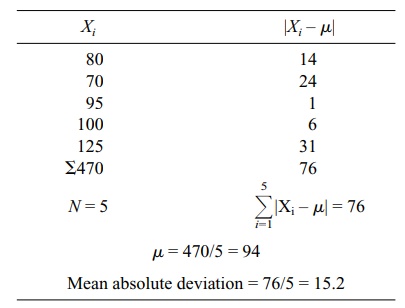
2. Mean Absolute Deviation

A second method we use to describe variability is called the mean absolute devi-ation. This measure involves first calculating the mean of a set of observations or values and then determining the deviation of each observation from the mean of those values. Then we take the absolute value of each deviation, sum all of the deviations, and calculate their mean. The mean absolute deviation for a sample is

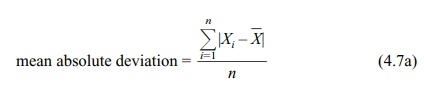
where n = number of observations in the data set.

The analogous formula for a finite population is

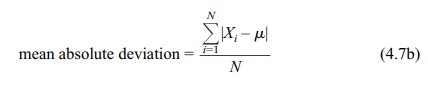
where N = number of observations in the population.

Here are some additional symbols and formulae. Let

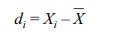
where:

X_i = a particular observation, 1 ≤ i ≤ n

 = sample mean

d_i = the deviation of a value from the mean

The individual deviations (d_i) have the mathematical property such that when we sum them

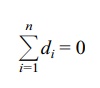
Thus, in order to calculate the mean absolute deviation of a sample, the formula must use the absolute value of d_i (|d_i|), as shown in Formula 4.7.

Suppose we have the following data set {80, 70, 95, 100, 125}. Table 4.5 demonstrates how to calculate a mean absolute deviation for the data set.

3. Population Variance and Standard Deviation

Historically, because of computational difficulties, the mean absolute deviation was not used very often. However, modern computers can speed up calculations of the mean absolute deviation, which has applications in statistical methods called robust procedures. 

TABLE 4.5. Calculation of a Mean Absolute Deviation (Blood Sugar Values for a Small Finite Population)

Common measures of dispersion, used more frequently because of their desirable mathematical properties, are the interrelated measures variance and standard deviation. Instead of using the absolute value of the deviations about the mean, both the variance and standard deviation use squared deviations about the mean, de-fined for the ith observation as (X_i – μ)². Formula 4.8, which is called the deviation score method, calculates the population variance (σ²) for a finite population. For in-finite populations we cannot calculate the population parameters such as the mean and variance. These parameters of the population distribution must be approximated through sample estimates. Based on random samples we will draw inferences about the possible values for these parameters.

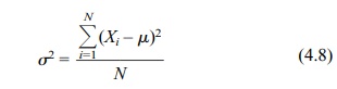
where N = the total number of elements in the population.

A related term is the population standard deviation (σ), which is the square root of the variance:

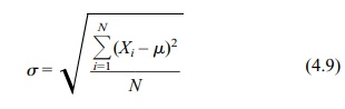
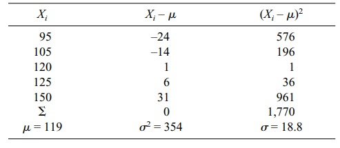
Table 4.6 gives an example of the calculation of σ for a small finite population.

The data are the same as those in Table 4.5 (μ = 94).

What do the variance and standard deviation tell us? They are useful for compar-ing data sets that are measured in the same units. For example, a data set that has a “large” variance in comparison to one that has a “small” variance is more variable than the latter one.

TABLE 4.6. Calculation of Population Variance

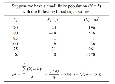
Returning to the data set in the example (Table 4.6), the variance σ² is 354. If the numbers differed more from one another, e.g., if the lowest value were 60 and the highest value 180, with the other three values also differing more from one another than in the original data set, then the variance would increase substantially. We will provide several specific examples.

In the first and second examples, we will double (Table 4.6a) and triple (Table 4.6b) the individual values; we will do so for the sake of argument, forgetting mo-mentarily that some of the blood sugar values will become unreliable. In the third example, we will add a constant, 25, to each individual value. The results are pre-sented in Table 4.6c.

TABLE 4.6a. Effect on Mean and Variance of Doubling Each Value of a Variable

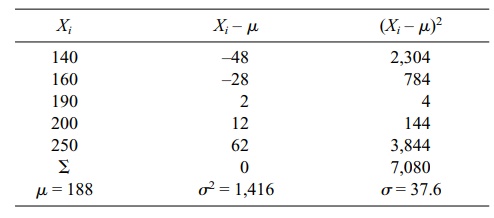
TABLE 4.6b. Effect on Mean and Variance of Tripling Each Value of a Variable

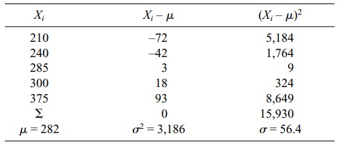
TABLE 4.6c. Effect on Mean and Variance of Adding a Constant (25) to Each Value of a Variable

What may we conclude from the foregoing three examples? The individual val-ues (X_i) differ more from one another in Table 4.6a and Table 4.6b than they did in Table 4.6. We would expect the variance to increase in the second two data sets be-cause the numbers are more different from one another than they were in Table 4.6; in fact, σ² increases as the numbers become more different from one another. Note also the following additional observations. When we multiplied the original X_i by a constant (e.g., 2 or 3), the variance increased by the constant squared (e.g., 4 or 9); however, the mean was multiplied by the constant (2 · X_i → 2μ, 4σ²; 3 · X_i → 3μ, 9σ²). When we added a constant (e.g., 25) to each X_i, there was no effect on the variance, although μ increased by the amount of the constant (25 + X_i → μ + 25; σ² = σ²). These relationships can be summarized as follows:

Effect of multiplying X_i by a constant a or adding a constant to X_i for each i:

1. Adding a: the mean μ becomes μ + a; the variance σ² and standard deviation σ remain unchanged.

2. Multiplying by a: the mean μ becomes μ a, the variance σ² becomes σ ²a², and the standard deviation σ becomes σ a.

The standard deviation also gives us information about the shape of the distribu-tion of the numbers. We will return to this point later, but for now distributions that have “smaller” standard deviations are narrower than those that have “larger” stan-dard deviations. Thus, in the previous example, the second hypothetical data set also would have a larger standard deviation (obviously because the standard deviation is the square root of the variance and the variance is larger) than the original data set. Figure 4.4 illustrates distributions that have different means (i.e., different locations) but the same variances and standard deviations. In Figure 4.5, the distributions have the same mean (i.e., same locations) but different variances and standard deviations.

4. Sample Variance and Standard Deviation

Calculation of sample variance requires a slight alteration in the formula used for population variance. The symbols S² and S shall be used to denote sample variance and standard deviation, respectively, and are calculated by using Formulas 4.10a and 4.10b (deviation score method).

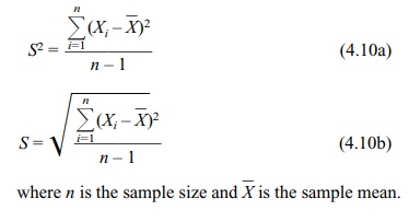
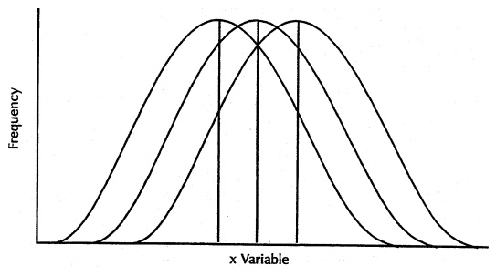
Figure 4.4. Symmetric distributions with the same variances and different means. (Source: Centers for Disease Control and Prevention (1992). Principles of Epidemiology, 2nd Edition, Figure 3.4)

Note that n – 1 is used in the denominator. The sample variance will be used to estimate the population variance. However, when n is used as the denominator for the estimate of variance, let us denote this estimate as S_m² · E(S_m²) ≠ σ², i.e., the ex-pected value of the estimate S_m² is biased; it does not equal the population variance. In order to correct for this bias, n–1 must be used in the denominator of the formula for sample variance. An example is shown in Table 4.7.

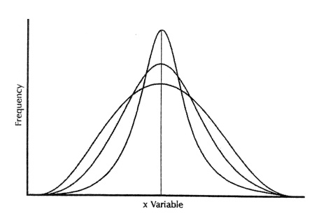
Figure 4.5. Distributions with the same mean and different variances. (Source: Centers for Disease Control and Prevention (1992). Principles of Epidemiology, 2nd Edition, Figure 3.4, p. 150.)

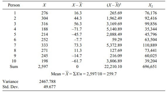
TABLE 4.7. Blood Cholesterol Measurements for a Sample of 10 Persons

Before the age of computers, finding the difference between each score and the mean was a cumbersome process. Statisticians developed a shortcut formula for the sample variance that is computationally faster and numerically more stable than the difference score formula. With the speed and high precision of modern computers, the shortcut formula is no longer as important as it once was. But it is still handy for doing computations on a pocket calculator.

This alternative calculation formula of sample variance (Formula 4.11) is algebraically equivalent to the deviation score method. The formula speeds the computation by avoiding the need to find the difference between the mean and each individual value:

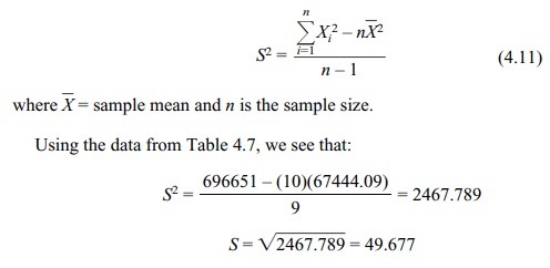
Using the data from Table 4.7, we see that:

S² = [696651 – (10)(67444.09)] / 9

 = 2467.789

S = √2467.789 = 49.677

5. Calculating the Variance and Standard Deviation from Grouped Data

For larger samples (e.g., above n = 30), the use of individual scores in manual cal-culations becomes tedious. An alternative procedure groups the data and estimates σ² from the grouped data. The formulas for sample variance and standard deviation for grouped data using the deviation score method (shown in Formulas 4.12a and b) are analogous to those for individual scores.

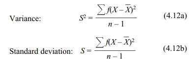
Table 4.8 provides an example of the calculations. In Table 4.8,  is the grouped mean [Σf X/Σf = 19188.50/373 ≈ 51.44 (by rounding to two decimal places)].