One-Compartment Open Model: Extravascular Administration

One-Compartment Open Model

Extravascular Administration

When a drug is administered by extravascular route (e.g. oral, i.m., rectal, etc.), absorption is a prerequisite for its therapeutic activity. Factors that influence drug absorption have already been discussed in chapter 2. The rate of absorption may be described mathematically as a zero-order or first-order process. A large number of plasma concentration-time profiles can be described by a one-compartment model with first-order absorption and elimination. However, under certain conditions, the absorption of some drugs may be better described by assuming zero-order (constant rate) kinetics. Differences between zero-order and first-order kinetics are illustrated in Fig. 9.6.

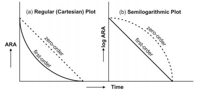
Fig. 9.6 Distinction between zero-order and first-order absorption processes. Figure a is regular plot, and Figure b a semilog plot of amount of drug remaining to be absorbed (ARA) versus time t.

Zero-order absorption is characterized by a constant rate of absorption. It is independent of amount remaining to be absorbed (ARA), and its regular ARA versus t plot is linear with slope equal to rate of absorption while the semilog plot is described by an ever-increasing gradient with time. In contrast, the first-order absorption process is distinguished by a decline in the rate with ARA i.e. absorption rate is dependent upon ARA; its regular plot is curvilinear and semilog plot a straight line with absorption rate constant as its slope.

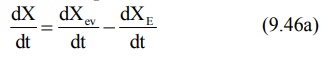
After e.v. administration, the rate of change in the amount of drug in the body dX/dt is the difference between the rate of input (absorption) dX_ev/dt and rate of output (elimination) dX_E/dt.

dX/dt = Rate of absorption – Rate of elimination

For a drug that follows one-compartment kinetics, the plasma concentration-time profile is characterized by absorption phase, post-absorption phase and elimination phase (Fig. 9.7.).

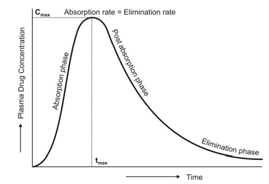
Fig. 9.7 The absorption and elimination phases of the plasma concentration-time profile obtained after extravascular administration of a single dose of a drug.

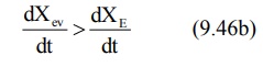
During the absorption phase, the rate of absorption is greater than the rate of elimination

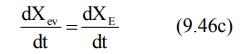
At peak plasma concentration, the rate of absorption equals the rate of elimination and the change in amount of drug in the body is zero.

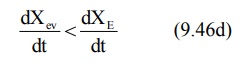
During the post-absorption phase, there is some drug at the extravascular site still remaining to be absorbed and the rate of elimination at this stage is greater than the absorption rate.

After completion of drug absorption, its rate becomes zero and the plasma level time curve is characterized only by the elimination phase.

a. Zero-Order Absorption Model

This model is similar to that for constant rate infusion.

The rate of drug absorption, as in the case of several controlled drug delivery systems, is constant and continues until the amount of drug at the absorption site (e.g. GIT) is depleted. All equations that explain the plasma concentration-time profile for constant rate i.v. infusion are also applicable to this model.

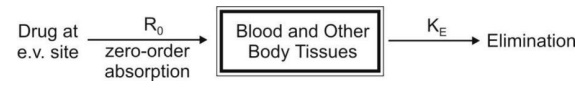
b. First-Order Absorption Model

For a drug that enters the body by a first-order absorption process, gets distributed in the body according to one-compartment kinetics and is eliminated by a first-order process, the model can be depicted as follows:

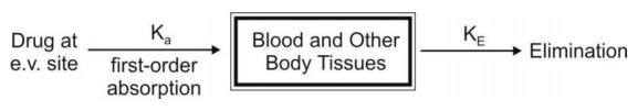
The differential form of the equation 9.46a is:

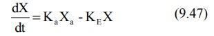
where,

K_a = first-order absorption rate constant, and

X_a = amount of drug at the absorption site remaining to be absorbed i.e. ARA.

Integration of equation 9.47 yields:

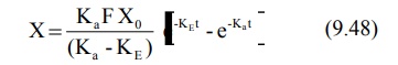
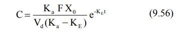
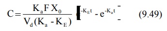
Transforming into concentration terms, the equation becomes:

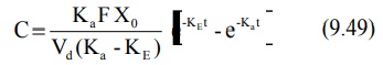
where F = fraction of drug absorbed systemically after e.v. administration. A typical plasma concentration-time profile of a drug administered e.v. is shown in Fig. 9.7.

Assessment of Pharmacokinetic Parameters

C_max and t_max: At peak plasma concentration, the rate of absorption equals rate of elimination i.e. K_aX_a = K_EX and the rate of change in plasma drug concentration dC/dt = zero. This rate can be obtained by differentiating equation 9.49.

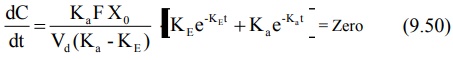
On simplifying, the above equation becomes:

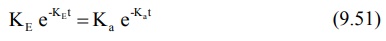
Converting to logarithmic form,

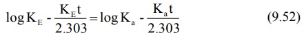
where t is t_max. Rearrangement of above equation yields:

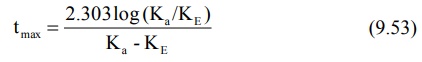
The above equation shows that as K_a becomes larger than K_E, t_max becomes smaller since (K_a – K_E) increases much faster than log K_a/K_E. C_max can be obtained by substituting equation 9.53 in equation 9.49. However, a simpler expression for the same is:

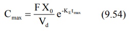
It has been shown that at C_max, when K_a = K_E, t_max = 1/K_E. Hence, the above equation further reduces to:

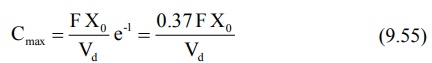
Since FX_o/V_d represents C_o following i.v. bolus, the maximum plasma concentration that can be attained after e.v. administration is just 37% of the maximum level attainable with i.v. bolus in the same dose. If bioavailability is less than 100%, still lower concentration will be attained.

Elimination Rate Constant: This parameter can be computed from the elimination phase of the plasma level time profile. For most drugs administered e.v., absorption rate is significantly greater than the elimination rate i.e. K_at >> K_Et. Hence, one can say that e^–Kat approaches zero much faster than does e^–KEt. At such a stage, when absorption is complete, the change in plasma concentration is dependent only on elimination rate and equation 9.49 reduces to:

Transforming into log form, the equation becomes:

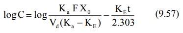
A plot of log C versus t yields a straight line with slope –K_E/2.303 (half-life can then be computed from K_E). K_E can also be estimated from urinary excretion data (see the section on urinary excretion data).

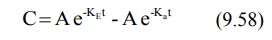
Absorption Rate Constant: It can be calculated by the method of residuals. The technique is also known as feathering, peeling and stripping. It is commonly used in pharmacokinetics to resolve a multiexponential curve into its individual components. For a drug that follows one-compartment kinetics and administered e.v., the concentration of drug in plasma is expressed by a biexponential equation 9.49.

If K_aFX_o/V_d(K_a-K_E) = A, a hybrid constant, then:

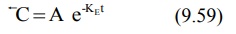
During the elimination phase, when absorption is almost over, K_a >> K_E and the value of second exponential e^–Kat approaches zero whereas the first exponential e^–KEt retains some finite value. At this time, the equation 9.58 reduces to:

In log form, the above equation is:

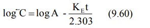
where C represents the back extrapolated plasma concentration values. A plot of log C versus t yields a biexponential curve with a terminal linear phase having slope –K_E/2.303 (Fig. 9.8). Back extrapolation of this straight line to time zero yields y-intercept equal to log A.

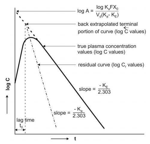
Fig. 9.8 Plasma concentration-time profile after oral administration of a single dose of a drug. The biexponential curve has been resolved into its two components— absorption and elimination.

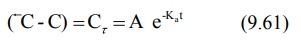
Subtraction of true plasma concentration values i.e. equation 9.58 from the extrapolated plasma concentration values i.e. equation 9.59 yields a series of residual concentration values C_r :

In log form, the equation is:

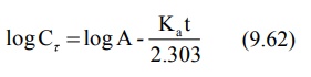
A plot of log C_r versus t yields a straight line with slope –K_a/2.303 and Y-intercept log A (Fig. 9.8). Absorption half-life can then be computed from K_a using the relation 0.693/K_a.

Thus, the method of residuals enables resolution of the biexponential plasma level-time curve into its two exponential components. The technique works best when the difference between K_a and K_E is large (K_a/K_E ≥ 3). In some instances, the K_E obtained after i.v. bolus of the same drug is very large, much larger than the K_a obtained by the method of residuals (e.g. isoprenaline) and if K_E/K_a ≥ 3, the terminal slope estimates K_a and not K_E whereas the slope of residual line gives K_E and not K_a. This is called as flip-flop phenomenon since the slopes of the two lines have exchanged their meanings.

Ideally, the extrapolated and the residual lines intersect each other on y-axis i.e. at time t = zero and there is no lag in absorption. However, if such an intersection occurs at a time greater than zero, it indicates time lag. It is defined as the time difference between drug administration and start of absorption. It is denoted by symbol t_o and represents the beginning of absorption process. Lag time should not be confused with onset time.

The above method for the estimation of K_a is a curve-fitting method. The method is best suited for drugs which are rapidly and completely absorbed and follow one-compartment kinetics even when given i.v. However, if the absorption of the drug is affected in some way such as GI motility or enzymatic degradation and if the drug shows multicompartment characteristics after i.v. administration (which is true for virtually all drugs), then K_a computed by curve-fitting method is incorrect even if the drug were truly absorbed by first-order kinetics. The K_a so obtained is at best, estimate of first-order disappearance of drug from the GIT rather than of first-order appearance in the systemic circulation.

Wagner-Nelson Method for Estimation of K_a

One of the better alternatives to curve-fitting method in the estimation of K_a is Wagner-Nelson method. The method involves determination of K_a from percent unabsorbed-time plots and does not require the assumption of zero- or first-order absorption.

After oral administration of a single dose of a drug, at any given time, the amount of drug absorbed into the systemic circulation X_A, is the sum of amount of drug in the body X and the amount of drug eliminated from the body X_E. Thus:

X_A = X + X_E                       (9.63)

The amount of drug in the body is X = V_dC. The amount of drug eliminated at any time t can be calculated as follows:

X_E = K_EV_d [AUC] ₀^t                   (9.64)

Substitution of values of X and X_E in equation 9.63 yields:

X_A = V_dC + K_EV_d [AUC]₀^t                 (9.65)

The total amount of drug absorbed into the systemic circulation from time zero to infinity X_A^∞ can be given as:

X_A^∞ = V_d C^∞ + K_E V_d [AUC]^∞₀             (9.66)

Since at t = ∞, C^∞ = 0, the above equation reduces to:

X^∞_A  = K_E V_d [AUC] ^∞₀                 (9.67)

The fraction of drug absorbed at any time t is given as:

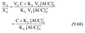
Percent drug unabsorbed at any time is therefore:

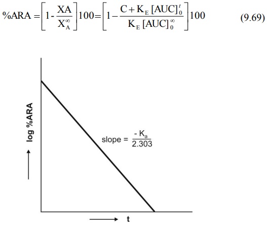
Fig. 9.9 Semilog plot of percent ARA versus t according to Wagner-Nelson method. Similar plot is obtained for Loo-Reigelman method

The method requires collection of blood samples after a single oral dose at regular intervals of time till the entire amount of drug is eliminated from the body. K_E is obtained from log C versus t plot and [AUC]o^t and [AUC] ^∞o are obtained from plots of C versus t. A semilog plot of percent unabsorbed (i.e. percent ARA) versus t yields a straight line whose slope is –K_a/2.303 (Fig.9.9). If a regular plot of the same is a straight line, then absorption is zero-order.

K_a can similarly be estimated from urinary excretion data (see the relevant section). The biggest disadvantage of Wagner-Nelson method is that it applies only to drugs with one-compartment characteristics. Problem arises when a drug that obeys one-compartment model after e.v. administration shows multicompartment characteristics on i.v. injection.

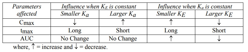
Effect of K_a and K_E on C_max, t_max and AUC

A summary of the influence of changes in K_a at constant K_E and of K_E at constant K_a on C_max, t_max and AUC of a drug administered e.v. is shown in Table 9.4.

TABLE 9.4

Influence of K_a and K_E on C_max, t_max and AUC

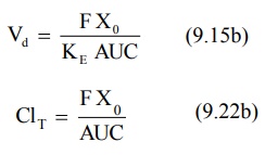
Apparent Volume of Distribution and Clearance: For a drug that follows one-compartment kinetics after e.v. administration, V_d and Cl_T can be computed from equation 9.15b and 9.22b respectively where F is the fraction absorbed into the systemic circulation.