Protein binding

Protein binding

A molecule (drug) that binds the protein is known as a ligand, and the protein with which it binds is called the substrate.

Protein binding is involved in the following:

·           Plasma protein binding of drugs in the central or plasma pharmacoki-netic compartment after administration.

·           Drug–receptor interactions (when the receptor is a protein) leading to drug action.

·           Substrate–enzyme interactions leading to enzyme action or inhibition.

Physical parameters of protein–ligand binding interaction include the kinet-ics of binding and its thermodynamics.

Kinetics of ligand–protein binding

Binding of a ligand (L) to a protein (P) to form a protein–ligand complex (PL) can be expressed as:

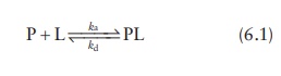
where, k_a and k_d are the equilibrium rate constants known as the associa-tion constant and the dissociation constant, respectively.

Their rate expressions can be written as:

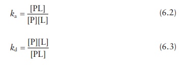
The dissociation constant (k_d) has a unit of concentration (such as M), while the association constant (k_a) has the unit of inverse concentration (such as M−1).

Thus,

k_d = 1/k_a                    (6.4)

1. Parameters of interest

Biopharmaceutical applications of protein binding require the determina-tion of two key parameters:

1. Binding affinity (defined as the association constant, k_a)

2. Binding capacity (maximum number of ligand molecules that can be bound per molecule of protein, y_max)

2. Experimental setup

Protein–ligand binding studies are usually carried out with fixed protein concentration and varying ligand concentration, or vice versa. At each con-centration, the amount of ligand bound is separated from free ligand by techniques such as centrifugation and filtration. Free ligand concentra-tion is then determined by analytical methods such as ultraviolet-visible spectroscopy (UV-VIS). The measurement of free ligand concentration as a function of total ligand concentration enables the determination of both the affinity and the capacity of ligand binding of the substrate.

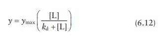
The amount of ligand bound to the substrate in each experiment (y) can be expressed as a fraction of maximum concentration that can be bound (y_max), as

Θ = y _/ y_max                (6.5)

Where, y represents the molar concentration, the amount of ligand bound per unit molar concentration, or the amount of protein, and y_max represents the maximum binding capacity.

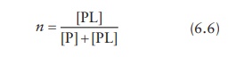
3. Determining k_a and y_max

Nonlinear regression I

Average number of ligand molecules bound per molecule of protein is expressed as the molar concentration of ligand bound to the protein per molar concentration of the protein. For the case of single binding site on the protein, molar concentration of ligand bound to the protein is given by [PL] and the total protein concentration is given by [P] + [PL]. Thus,

From the expression for the dissociation constant, k_d,

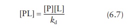
Combining these two equations,

For a single ligand-binding site per protein,

n = θ                    (6.9)

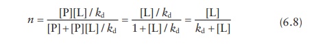
Thus, the amount of ligand bound to the protein as a fraction of sat-uration concentration (θ), which is experimentally determined, can be written as:

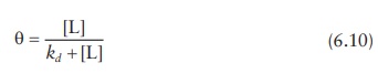
Directly plotting θ against the free ligand concentration [L] gives a satura-tion curve (Figure 6.8a), and the data can be fitted by nonlinear regression to solve for y_max and k_d as parameters.

However, nonlinear regression is a computationally intensive parameter-estimation method that uses algorithms for adjusting the equation parameters to best fit the data. Thus, it suffers the drawbacks of requiring software support, being dependent on the initial values of parameters chosen, and the possibility of coming up with incorrect parameters due to minimization of sum-of-square errors in a local region. Therefore, lineariza-tion of this equation followed by simple linear regression is traditionally preferred. Two methods for linearization are the double-reciprocal plot and the Scatchard plot.

Linear regression I: Double-reciprocal (Hughes–Klotz) plot

Inverting Equation 6.11,

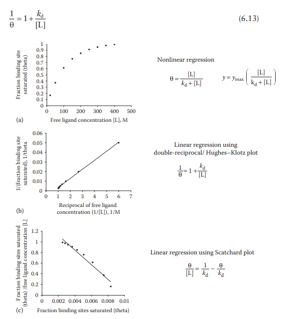
Figure 6.8 Methods for determining ligand–protein interaction parameters.

In this equation, [L] represents the free ligand concentration, which is also experimentally determined. This is a linear form of the equation, whereby plotting 1/θ against 1/[L] gives a straight line, with slope as k_d. This plot is known as the double-reciprocal plot, Lineweaver– Burk plot, Benesi–Hildebrand binding curve, or the Hughes–Klotz plot (Figure 6.8b).

As seen in Figure 6.8b, graphical treatment of data using Klotz reciprocal plot heavily weighs those experimental points obtained at low concentrations of free ligand and may, therefore, lead to misinter-pretations regarding the protein-binding behavior at high concentrations of free ligand. The Scatchard plot (Figure 6.8c)—discussed in the next section—does not have this disadvantage and is, therefore, preferred for plotting data.

Linear regression II: Scatchard plot

The equation for θ can also be converted into:

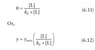
Adding and subtracting 1/k_d from this equation:

Thus, given that both θ and [L] are experimentally determined, plotting θ/[L] against θ would give a slope of −1/k_d and an intercept of y_max/k_d. This linear plot is known as the Scatchard plot (Figure 6.8c). Interchanging the x- and y-axis of the Scatchard plot results in the Eadie–Hofstee plot.

Although the Scatchard plot is widely used for protein–ligand bind-ing data analyses, it suffers from mathematical limitations. As seen in Figure 6.8c, the Scatchard transformation distorts experimental error, resulting in violation of the underlying assumptions of linear regression, viz., Gaussian distribution of error and standard deviations being the same for every value of the known variable. In addition, plotting θ/[L] against θ leads to the unknown variables being a part of both x- and y-axis, while linear regression assumes that y-axis is unknown and x-axis is precisely known.

Thermodynamics of ligand–protein binding

Binding affinity can also be inferred from the thermodynamics of binding. A binding interaction, where more stable bonds are formed than are broken, involves release of energy as heat. The amount of heat released can be pre-cisely measured in carefully controlled experiments by a technique generally known as calorimetry. For example, isothermal titration calorimetry (ITC) involves the titration of one binding partner (ligand) into another (protein) while measuring the heat (enthalpy) change per unit volume of the ligand added to the protein. These data are integrated to yield enthalpy change per mole of the injectant and plotted against the molar ratio of ligand to protein (Figure 6.9). In this plot, the enthalpy difference between the starting value and the saturated value indicates enthalpy (∆H) of binding, the slope of the transition indicates binding affinity, and the ligand/protein molar ratio at the inflexion point indicates the stoichiometry of binding, that is, the num-ber of ligand molecules binding per protein molecule.

Thus, ITC can be used to determine the thermodynamic parameters associated with a physical or a chemical change. These parameters include the free energy (∆ G), enthalpy (∆ H), and entropy (∆ S) change, which are related to each other as:

∆G= ∆H−T∆S

Spontaneous processes must have favorable overall free energy of reaction (negative ∆ G). The ITC helps determine whether the ligand–protein binding is enthalpically driven (negative ∆ H) or entropically driven (positive ∆ S).

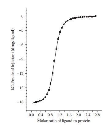
Figure 6.9 A typical ITC thermogram.

An entropically driven process is likely to be significantly influenced by the liquid medium. In the case of an enthalpically driven process, the binding constant and the enthalpy change associated with the binding are indicative of the strength of binding. Complexation is a binding process whereby the degrees of freedom of two or more molecules are reduced as they bind each other. Thus, complexation is an entropically unfavorable process (i.e., has a negative entropy).

An ITC experiment can also help determine the dissociation constant (k_d).

ΔG = −RT lnk_d                    (6.17)

where:

R is the gas constant

T is the absolute temperature

Factors influencing protein binding

The physicochemical characteristics and concentration of the drug, the pro-tein, and the characteristics of the liquid medium in which binding takes place influence drug (ligand)–protein binding.

1. Physicochemical characteristics and concentration of the drug

The extent of protein binding of many drugs is a linear function of their oil–water partition coefficient (Figure 6.10), which is a measure of their hydrophobicity. Thus, protein binding generally increases with an increase in drug lipophilicity. This indicates involvement of drug– protein hydrophobic interactions. This phenomenon can be used to predict the biological activity of a drug’s analogs. For example, an increase in the

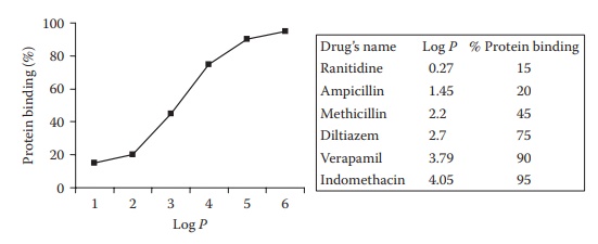
Figure 6.10 Effect of lipophilicity (log P) on plasma protein binding of drugs.

lipophilicity of penicillins results in decreased activity. The hydrophobic binding of penicillin in serum proteins reduces their potency in vivo, by decreasing their free plasma concentration.

Increasing the concentration of the drug would generally increase the extent of binding. However, if the concentration is increased beyond the saturation concentration, saturation of some or all binding sites can occur and the proportion of drug bound would actually decrease, as the absolute amount of bound drug remains constant.

2. Physicochemical characteristics and concentration of the protein

In a dilute solution, increasing protein concentration is expected to increase the proportion of the drug bound. However, at high protein concentrations, the protein may agglomerate or self-associate, leading to shielding of the hydrophobic region(s), which can reduce drug binding if the drug—protein interaction is driven by hydrophobic interactions.

Physicochemical characteristics of the protein, such as the density dis-tribution of hydrophobic groups on its surface, significantly influence the extent of drug–protein interaction. Thus, binding affinity of a drug toward different proteins can be markedly different.

3. Physicochemical characteristics of the medium

Binding interaction between the drug and the protein involves disruption of drug–solvent and protein–solvent bonds with the formation of drug– protein bonds. Thus, solvent medium that strongly interacts with either or both of the drug and protein can lead to thermodynamically unfavorable outcome of drug–protein interactions. In addition, change in the dielectric constant of the medium, such as in the presence of alcohol in aqueous solutions, can lead to altered forces of attraction and bonding between the drug and the protein. For example, salt concentration and dielectric constant of the solvent medium can significantly influence drug–protein interactions.

Plasma protein binding

Systemically administered drugs reach target organs and tissues through blood, which is a mixture of several substances, including proteins. In pharmacokinetic terms, the blood or the plasma is called the central com-partment. In this compartment, drugs often bind plasma proteins. The drug exits the central compartment as it partitions into organs and tissues, called the peripheral compartment. Plasma protein binding of drugs is generally reversible, so that protein-bound drug molecules are released as the level of free drug in blood declines.

1. Plasma proteins involved in binding

Blood plasma normally contains about 6.72 g of protein per 100 cm³, the protein comprising 4.0 g of albumin, 2.3 g globulin, and 0.24 g of fibrinogen. Albumin (commonly called human serum albumin [HSA]) is the most abundant protein in plasma and interstitial fluid. Plasma albumin is a globular protein consisting of a single polypeptide chain of molec-ular weight 67 kDa. It has an isoelectric point of 4.9 and, therefore, a net negative charge at pH 7.4. Nevertheless, albumin is amphoteric and capable of binding both acidic and basic drugs. Physiologically, it binds relatively insoluble endogenous compounds, including unesterified fatty acids, bilirubin, and bile acids. Human serum albumin has two sites for drug binding:

1. Site I (warfarin site) binds bilirubin, phenytoin, and warfarin.

2. Site II (diazepam site) binds benzodiazepines, probenecid, and ibuprofen.

Plasma proteins other than albumin are sometimes the major binding part-ners of drugs. For example, dicoumarol is bound to β- and α-globulins, and certain steroid hormones are specifically and preferentially bound to particular globulin fractions. Among other proteins, α1-acid glycoprotein (AAG) binds to lipophilic cations, including promethazine, amitriptyline, and dipyridamole.

2. Factors affecting plasma–protein binding

The amount of a drug that is bound to plasma proteins depends on three factors:

1. Concentration of free drug

2. Drug’s affinity for the protein-binding sites

3. Concentration of protein

3. Consequences of plasma–protein binding

The binding of drugs to plasma proteins can influence their action in a number of ways:

1. Reduce free drug concentration. Protein binding affects antibiotic effectiveness, as only the free antibiotic has antibacterial activity. For example, penicillin and cephalosporins bind reversibly to albumin, thus affecting their free concentrations in plasma.

2. Reduce drug diffusion. The bound drug assumes the diffusional and other transport characteristics of the protein molecules.

3. Reduce volume of distribution. Only free drug is able to cross the pores of the capillary endothelium. Protein binding will affect drug transport into other tissues. When binding occurs with high affinity, the drug is preferentially localized in the plasma or the central com-partment. In pharmacokinetic measurements, this reflects as a low volume of distribution of the drug.

However, some drugs (e.g., warfarin and tricyclic antidepressants) may exhibit both a high degree of PPP and a large volume of distri-bution. Although drug bound to plasma proteins is not able to cross biological membranes, binding of drugs to plasma proteins is in a dynamic equilibrium with the drug bound to plasma proteins. If the unbound (or free) drug is able to cross biological membranes and has a greater affinity and capacity for binding to the tissue biomolecules, compared with the plasma proteins, the drug may exhibit high vol-ume of distribution, despite also exhibiting high PPP. As free drug moves across membranes and out of vascular space, the equilibrium shifts, drawing drug off the plasma protein to replenish the free drug lost from vascular space. This free drug is now also able to traverse membranes and leave vascular space. In this way, a drug with a very low free fraction (i.e., a high degree of PPP) can exhibit a large volume of distribution.

4. Reduce elimination. Protein binding retards the metabolism and renal excretion of the drug. Proteins are not filtered through glomerular filtration. Thus, protein-bound drugs have reduced rate of filtration in the kidneys and metabolism in the liver.

5. Increase risk of fluctuation in plasma free drug concentration.

a. In cases where a drug is highly protein-bound (around 90%), small changes in binding, protein concentration, or displacement of the drug by another coadministered drug (drug–drug interaction) can lead to drastic changes in the concentration of free drug in the body, thus affecting efficacy and/or toxicity.

However, a plasma protein may have multiple binding sites. Thus, if drugs bind to different sites on a protein, there will not be a competitive binding interaction between them. Thus, some drugs that are highly bound to albumin exhibit competitive inter-actions, while others do not.

b. Sometimes, drug administration may also cause displacement of body hormones that are physiologically bound to the protein, thus increasing free hormone concentration in the blood.

c. Disease states that alter plasma protein concentration may alter the protein binding of drugs. If the concentration of protein in plasma is reduced, there may be an increase in the free fraction of the drugs bound to that protein. Similarly, if pathological changes in binding proteins reduce the affinity of drug for the protein, there will be an increase in the free fraction of drug.

Effect on dosing regimen

Plasma protein binding can affect dosing regimen of a drug in several ways.

1. Lower metabolism and elimination of a plasma-protein-bound drug can lead to longer plasma half-life, compared with an unbound drug. Thus, the protein-bound drug may serve as a reservoir of drug within the body, maintaining free drug concentration through equilibrium dissociation process. This leads to long half-life and sustained plasma concentrations. Thus, dosing frequency would need to be adjusted in cases where drug’s PPP or the concentration of plasma proteins is affected (such as burns).

2. Dose adjustments are frequently required in the case of disease states that affect the protein to which the administered drug is bound. Certain disease states increase AAG concentration while reducing albumin concentration. For example, acute burns reduce the con-centration of circulating albumin, resulting in an increase in the free fraction of drugs that are normally bound to albumin. On the other hand, AAG concentration is substantially increased after an acute burn, resulting in a decrease in the free fraction of drugs that are normally bound to this plasma protein.

3. Age-based dose adjustments often have to account for PPP of drugs. For example, newborns have selectively lower plasma protein levels than adults. Thus, although the neonatal HSA concentration at birth is 75%–80% of adult levels, AAG concentration is only ~50%. Thus, dose adjustment may be needed for drugs that bind AAG.

4. Drug–drug interactions. Drugs that compete for the same plasma-protein-binding site can displace one another. This can lead to increased free level of a drug. Minor perturbation in PPP can have a significant influence on free drug concentration. Thus, coadministration of cer-tain drugs may be contraindicated or require dose adjustment.

Drug receptor binding

Target protein (receptor) binding is routinely utilized in drug discovery, with the goal of maximizing binding affinity and specificity. This is expected to result in a drug molecule that is highly potent and has low off-target activ-ity and, thus, toxicity. The principles involved in delineating the kinetics of drug–receptor binding are same as discussed earlier for ligand–protein binding.

Substrate enzyme binding

Binding of a ligand, which serves as a substrate for an enzyme, to an enzyme is a part of a continuous process involving conversion of the substrate into the product(s) by the enzyme. This process involves continuous recycling of the enyzme’s binding sites for fresh substrate, as each molecule of the substrate is converted into product(s). Thus, substrate–enzyme binding kinetics are represented in terms of the rate of binding, and the satura-tion of the binding kinetics is considered in terms of the maximum rate of binding.

The rate of binding kinetics for substrate–enzyme reactions follows a hyperbolic function, described by the Michaelis–Menten equation.

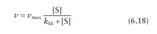
where:

v is the initial reaction rate

v_max is the maximum reaction rate

[S] is the substrate concentration

k_M is the Michaelis–Menten constant, which represents the ratio of the rate of dissociation of the enzyme–substrate complex to its rate of formation.

The similarity of this equation to Equation 6.7 indicates similar basic prin-ciples involved in their derivation.