Exercises questions answers
| Home | | Advanced Mathematics |Chapter: Biostatistics for the Health Sciences: Estimating Population Means
Biostatistics for the Health Sciences: Estimating Population Means - Exercises questions answers
EXERCISES
8.1 In your own words define the following terms:
a. Descriptive statistics
b. Inferential statistics
c. Point estimate of a population parameter
d. Interval (confidence interval) estimate of a population parameter
e. Type I error
f. Biased estimator of a population parameter
g. Mean square error
8.2 What are the desirable properties of an estimator
of a population parameter?
8.3 What are the advantages and disadvantages of using
point estimates for sta-tistical inference?
8.4 What are the desirable properties of a confidence
interval? How do sample size and the level of confidence (e.g., 90%, 95%, 99%)
affect the width of a confidence interval?
8.5 State the advantages and disadvantages of using
confidence intervals for sta-tistical inference.
8.6 Two situations affect the choice of a calculation
of a confidence interval: (1) the population is known; (2) the population
variance is unknown. How would you calculate a confidence interval given these
two different circumstances?
8.7 Explain the bootstrap principle. How can it be
used to make statistical infer-ences?
8.8 How can bootstrap confidence intervals be
generated? Name the simplest form of a bootstrap confidence interval. Are
bootstrap confidence intervals exact?
8.9 Suppose we randomly select 20 students enrolled in
an introductory course in biostatistics and measure their resting heart rates.
We obtain a mean of 66.9 (S = 9.02).
Calculate a 95% confidence interval for the population mean and give an interpretation
of the interval you obtain.
8.10 Suppose that a sample of pulse rates gives a mean
of 71.3, as in Exercise 8.9, with a standard deviation that can be assumed to
be 9.4 (close to the estimate observed in exercise 8.9). How many patients
should be sampled to obtain a 95 % confidence interval for the mean that has
half-width 1.2 beats per minute?
8.11 In a sample of 125 experimental subjects, the mean
score on a postexperi-mental measure of aggression was 55 with a standard
deviation of 5. Con-struct a 95% confidence interval for the population mean.
8.12 Suppose the sample size in exercise 8.11 is 169
and the mean score is 55 with a standard deviation of 5. Construct a 99%
confidence interval for the popu-lation mean.
8.13 Suppose you want to construct a 95% confidence
interval for mean aggres-sion scores as in Exercise 8.11, and you can assume
that the standard devia-tion of the estimate is 5. How many experimental
subjects do you need for the half-width of the interval to be no larger than 0.4?
8.14 What would the number of experimental subjects
have to be under the as-sumptions in Exercise 8.13 if you want to construct a
99% confidence inter-val with half-width no greater then 0.4? Under the same
criteria we decide that n should be
large enough so that a 95% confidence interval would have this half-width of
0.4. Which confidence interval requires the larger sample size and why? What is
n for the 95% interval?
8.15 The mean weight of 100 men in a particular heart
study is 61 kg with a stan-dard deviation of 7.9 kg. Construct a 95% confidence
interval for the mean.
8.16 The standard hemoglobin reading for normal males
of adult age is 15 g/100 ml. The standard deviation is about 2.5 g/100 ml. For
a group of 36 male con-struction workers, the sample mean was 16 g/100 ml.
a. Construct a 95% confidence interval for the male construction workers.
What is your interpretation of this interval relative to the normal adult male
population?
b. What would the confidence interval have been if the above results were obtained
based on 49 construction workers?
c. Repeat b for 64 construction
workers.
d. Do fixed-level confidence intervals shrink or widen as the sample size
in-creases (all other factors remaining the same)? Explain your answer.
e. What is the half-width of the confidence interval that you would obtain
for 64 workers?
8.17 Repeat Exercise 8.16 for 99% confidence intervals.
8.18 The mean diastolic blood pressure for 225 randomly
selected individuals is 75 mmHg with a standard deviation of 12.0 mmHg.
Construct a 95% confi-dence interval for the mean.
8.19 Change exercise 8.18 to assume there are 400
randomly selected individuals with a mean of 75 and standard deviation of 12.
Construct a 99% confidence interval for the mean.
8.20 In Exercise 8.18, how many individuals must you
select to obtain the half-width of a 99% confidence interval no larger than 0.5
mmHg?
Answer:
8.2 A point estimate is a single value intended to
approximate a population para-meter. An unbiased estimate is an estimate or a
function of observed random vari-ables that has the property that the average
of its sampling distribution is equal to the population parameter, whatever
that value might be. Unbiasedness is a desirable property but the key for an
estimator is accuracy. Unbiased estimators with small variance are desirable
but an unbiased estimator with a large variance is not if other estimates can
be found that are more accurate. The mean square error is a measure of
accuracy. It penalizes an estimate for both bias and variance. An estimate with
small mean square error tends to be close to the true parameter value.
8.7 The bootstrap principle states that we can
approximate the sampling distribu-tion of a point estimate by mimicking the
random sample we observe to compute the estimate. The bootstrap estimates are
obtained by sampling with replacement from the observed data. Bootstrap
sampling mimics the random sampling of the original data. The original sample
replaces the population and the bootstrap sample replaces the original sample.
The bootstrap estimates are obtained by applying the function of the
observations to the bootstrap sample. The distribution of these bootstrap
esti-mates is used as an approximation to the sampling distribution for the
estimate.
8.8 The bootstrap confidence intervals are obtained by
generating bootstrap samples by the Monte Carlo approximation. The histogram
of values of the bootstrap estimates can then be used to generate confidence
intervals. One of the simplest of bootstrap confidence intervals is called
Efron’s percentile method. It constructs a 100(1 – a)%
confidence interval by taking the lower endpoint to be the 100(a/2) percentile and the upper endpoint to be the 100(1 – a/2) percentile.
8.10 We need to find
C, the 97.5 percentage point from
the t distribution with n –
1 degrees of freedom such that Cσ/√n
≤ d. Here d = 1.2 and S = 9.4. So we need to find the smallest
n such that n ≥ C2S2/d2 = C2(61.36). From the table of Student’s t distribution, we see the results in
the following table:
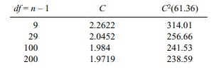
From the table, we see that n > 235, since for n =
235, C > 1.96 and (1.96)2(61.36)
= 235.72. Also, C < 1.9719 for n = 235, so for n = 235, 235.72 < C2(61.36)
< 238.59. Now 239 is clearly large enough.
8.14 Since the mean score is 55 and the standard deviation
is 5, we want to find n
so that the half-width of a 99% confidence interval for the population mean
has a half-width d no greater than
0.4. Again, n must satisfy n ≥ C2S2/d2 = C2(156.25),
where C is the 99.5 percentile of a t distribution with n – 1 degrees of freedom. We use the following table:
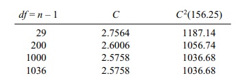
After df
= 200, the value of C is close enough
to the limiting normal value that we use the limiting value of 2.5758. We see
that we need df = 1036 or n = 1037 to meet our requirement. For a
95% confidence interval with the same mean and standard deviation, we would
require a smaller n for the same d = 0.4 since the constant C is smaller—1.96 compared to 2.5758. We
reduce the sample size by lowering the lev-el of confidence. We still require n ≥ C2S2/d2 = C2(156.25)
but now since C = 1.96, we have n > 600.25 or n = 601.
8.16 a. We have assumed that the standard deviation is
known to be 2.5. A 95% confidence
interval for 36 construction workers would then be [16 – (1.96) (2.5)/√36, 16 + (1.96)(2.5)/ √36] = [15.1833, 16.8167].
b. Had n been 49, we just replace √36 = 6 by
√49 = 7. This gives [16 – (1.96) (2.5)/7, 16 + (1.96)(2.5)/7] = [15.3,
16.7].
c. Now if n = 64 we replace 7 by 8 = √64 to get
[16 – (1.96)(2.5)/8, 16 + (1.96)(2.5)/8] = [15.3875, 16.6125].
d. As we see from a through c we
kept the level the same and we found that the width continued to decrease as
the sample size increased. With each new interval being contained in the
previous one (since the mean and standard deviation did not change). This just
illustrates that the width of the interval, which is a constant divid-ed by the
square root of the sample size, decreases because the square root of the sample
size increases as the sample size increases.
e. The halfwidth of the interval in c is 0.6125 =
(1.96)(2.5)/8.
Related Topics
