Confidence Intervals for the Difference between Means from Two Independent Samples (Variance Unknown)
| Home | | Advanced Mathematics |Chapter: Biostatistics for the Health Sciences: Estimating Population Means
Biostatistics for the Health Sciences: Estimating Population Means - Confidence Intervals for the Difference between Means from Two Independent Samples (Variance Unknown)
CONFIDENCE INTERVALS FOR THE DIFFERENCE BETWEEN MEANS FROM TWO
INDEPENDENT SAMPLES (POPULATION VARIANCE UNKNOWN)
In the case when the variances of the parent
populations from which the samples are selected are unknown, we use the t statistic with the pooled variance
formula from Section 8.5 assuming normal distributions and equal variances.
When the variances are assumed to be unequal and the distributions normal, we
use the k statistic from Section 8.5
with the individual sample variances. When using k, we apply the Welch–Aspin t
approximation with v degrees of freedom where v is defined as in Section 8.5.
In the first case the 95% confidence interval is
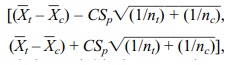
,
where Sp is the pooled estimate of the standard deviation and C is the appropriate constant such that P(–C
≤ t ≤ C) = 0.95 when t has a
Student’s t distribution with nt + nc – 2 degrees of freedom. The formula for the 95%
confidence interval for the difference between two population means assuming
unknown and common population variances is given in Display 8.5.
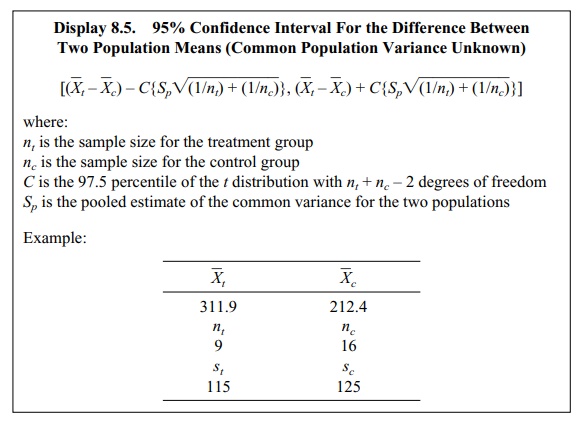
Now recall that Sp2
= {S2t(nt
– 1) + Sc2(nc – 1)/[nt + nc
– 2]}; Sp2 =
{(115)2(8) + (125)2(15)}/(9 + 16–2) = {13225(8) + 15625
(15)}/23 = {105800 + 2343750/23} = 340175/23 = 14790.22. Sp is the square root of 14790.22 = 121.62. So the
interval is
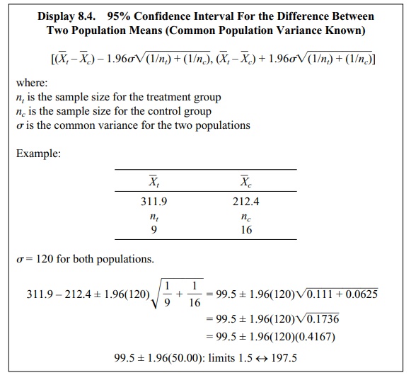
Display 8.4. 95% Confidence Interval For the Difference Between Two
Population Means (Common Population Variance Known)
as follows:

From the t
table we see that C = 2.0687 since
the degrees of freedom are 23. Using this value for C we get the following:
[99.5–2.0687{121.62 √[(1/9) + (1/16)]}, 99.5 + 2.0687{121.62 √ [(1/9) +
(1/16)]}]
= [99.5–249.53(0.1736, 99.5 + 249.53(0.1736] =
= [99.5–249.53(0.4167), 99.5 + 249.53(0.4167)] =
= [99.5–103.98, 99.5 + 103.98] = [–4.48, 203.48]
In the second case, the 95% confidence interval is
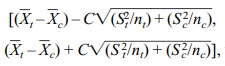 ,
,
where S2t is the sample estimate of variance for the treatment group and Sc2 is the sample estimate of variance for the control group. The quantity C is calculated such that P(–C ≤ k ≤ C) = 0.95 when k has Student’s t distribution with v degrees of freedom. Refer to Display 8.6 for the formula for a 95% confidence interval for a difference between two population means, assuming differ-ent unknown population variances.
Display 8.5. 95% Confidence Interval
For the Difference Between Two Population Means (Common Population Variance
Unknown)
Let us consider an example from the pharmaceutical
industry. A company is in-terested in marketing a clotting agent that reduces
blood loss when an accident causes an internal injury such as liver trauma. To
study possible doses of the agent and obtain some indication of safety and
efficacy, the company conducts an experiment in which a controlled liver
injury is induced in pigs and blood loss is mea-sured. Pigs are randomized as
to whether they receive the drug after the injury or do not receive drug
therapy—the treatment and control groups, respectively.
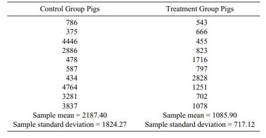
The following data were taken from a study in which
there were 10 pigs in the treatment group and 10 in the control group. The
blood loss was measured in milli-liters and is given in Table 8.1.
When the variances are known, we use the Z statistic defined in the previous
section, namely
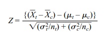
Z has exactly the standard normal distribution when
the observations in both sam-ples are normally distributed. Also, based on the
central limit theorem, Z is
approx-imately normal if conditions for the central limit theorem are satisfied
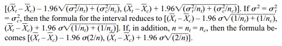
for each population being sampled. So for a 95% confidence interval we know
that P(–C ≤ Z ≤ C) = 0.95 if C = 1.96. So  1.96). After some algebra we find that
TABLE 8.1. Pig Blood Loss Data (ml)
So the 95% confidence interval is
For
other confidence levels we just change the constant C to 1.645 for 90% or 2.575 for 99%.
For these data, we note a large difference between
the sample standard devia-tions: 717.12 for the treatment group versus 1824.27
for the control group. This result is not compatible with the assumption of
equal variance. We will make the as-sumption anyway to illustrate the
calculation. We will then revisit this example and calculate the confidence
interval obtained, dropping the equal variance assumption and using the t approximation with the k statistic. In Section 8.9, we will
look at the result we would obtain from a bootstrap percentile method
confidence interval where the questionable normality assumption can be dropped.
In Chapter 9, we will look at the conclusions of various hypothesis tests based
on these pig blood loss data and various assumptions about the population
variances. We will revisit the ex-ample one more time in Section 14.3, where we
will apply a nonparametric tech-nique called the Wilcoxon rank–sum test to
these data.
Using the formula for the estimated common variance (Display 8.5), we must calculate the pooled variance S p2. The term S 2p = {S2t(nt – 1) + Sc2(nc – 1)}/[nt + nc – 2] = {(717.12)2 9 + (1824.27)2 9}/18, where nt = nc = 10, St = 717.12, and Sc = 1824.27. So Sp2 = 2178241.61; taking the square root we obtain Sp = 1475.89. Since the degrees of freedom are nt + nc – 2 = 18, we find that the constant C from the table of the Student’s t distribution is 2.101.
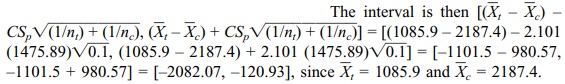
In Chapter 9 (on
hypothesis testing), you will learn that because the interval does not contain
0, you are able to reject the hypothesis of no difference in average blood
loss.
We note that if we had chosen a 90% confidence
interval C = 1.7341 (based on the tables for Student’s t distribution), the
resulting interval would be [(1085.9 – 2187.4) – 1.7341(1475.89) √0.1, (1085.9 – 2187.4) + 1.7341(1475.89) √0.1] =
[–1101.5 – 809.33, –1101.5 + 809.33] = [–1910.83, –292.17].
Now let us look at the result obtained from
assuming unequal variances, a more realistic assumption (refer to Display 8.6).
The confidence interval would then be 
, where C is obtained from a
Student’s t distribution with v
degrees of freedom and
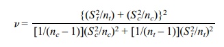
Using St
= 717.12 and Sc = 1824.27,
we obtain v = 11.717. Note that we cannot look up C in the t table since
the degrees of freedom (v) are not an
integer. Interpo-lation of results for 11 and 12 degrees of freedom (a linear
approximation for de-grees of freedom between 11 and 12) could be used as an
approximation to C. It can also be
calculated numerically. For 11 degrees of freedom C = 2.201. For 12 de-grees of freedom C = 2.1788. The interpolation formula is as follows:
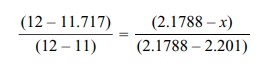
We solve for x
as the interpolated value for C. The
simple way to remember the change in degrees of freedom from 12 to 11.717 is to
define the change in degrees of freedom from 12 to 11 as the change in C from the value for 12 degrees of free
So taking C = 2.185, the 95% confidence interval is [(1085.9 – 2187.4) – 2.185 √332796.1, (1085.9 – 2187.4) + 2.185√332796.1] = [–1101.5 – 1260.49, –1101.5 + 1260.49] = [–2361.99, 158.99].
We note that this interval is different from the previous calculation for the com-mon variance estimate and perhaps more realistic. The conclusion is also qualita-tively different from the previous calculation because in this case the interval con-tains 0, whereas under the equal variance assumption it did not!
Display 8.6. A 95% Confidence
Interval for a Difference Between two Population Means (Different Unknown
Population Variances)

where:
nt is the sample size for the treatment group
S2t is the sample
estimate of variance for the treatment group
nc is the sample size for the control group
Sc2 is the sample
estimate of variance for the control group
C is the 97.5
percentile of the t distribution with v degrees of freedom with v given by
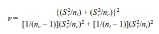
Related Topics
