Confidence Intervals for a Single Population Mean

CONFIDENCE INTERVALS FOR A SINGLE POPULATION MEAN

To understand how confidence intervals work, we will first illustrate them by the simplest case, in which the observations have a normal distribution with a known variance σ² and we want to estimate the population mean, μ. Then we know that the sample mean is  and its sampling distribution has mean equal to the population  mean μ and a variance σ ²/n, where n is the number of samples. Thus, Z = (– μ)/( σ /√n) has a standard normal distribution. We can therefore state that P(–1.96 ≤ Z ≤ 1.96) = 0.95 based on the standard normal distribution. Substituting ( – μ)/(σ/√n) for Z we obtain P(–1.96 ≤ ( – μ)/(σ/√n) ≤ 1.96) = 0.95 or P(–1.96σ/√n ≤ ( – μ) ≤ 1.96σ/√n) = 0.95 or P(–1.96(σ/√n) –  ≤ – μ ≤ 1.96(σ/√n) – ) = 0.95. Multiplying throughout by –1 and reversing the inequality, we find that P(1.96(σ/√n) +  ≥ μ ≥ –1.96(σ/√n) + ) = 0.95. Rearranging the foregoing formula, we have P( – 1.96σ/√n ≤ μ ≤ X + 1.96σ/√n) = 0.95. The confidence interval is an interpretation of this probability statement. The confidence interval [– 1.96σ/√n, X + 1.96σ/√n] is a random interval determined by the sample value of  , σ, n, and the confidence level (e.g., 95%).  is the component to this interval that makes it random. (See Display 8.2.)

The probability statement P [ – 1.96(σ/√n) ≤ μ ≤  + 1.96(σ/√n)] = 0.95 says only that the probability that this random interval includes the population mean is 0.95. This probability pertains to the procedure for generating random confidence intervals. It does not say what will happen to the parameter on any particular out-come. If, for example, σ is 5 and n = 25 and we obtain from a sample a sample mean of 5.96, then the outcome for the random interval is [5.96 – 1.96, 5.96 + 1.96] = [4.00, 7.92]. The population mean will either be inside or outside the interval. If the mean μ = 7, then it is contained in the interval. On the other hand, if μ = 8, μ is not contained in the interval.

We cannot say that the probability is 0.95 that the single fixed interval [4.00, 7.92] contains μ. It either does or it does not. Instead, we say that we have 95% confidence that such an interval would include (or cover) μ. This means that the process will tend to include the true value of the parameter 95% of the time if we

Display 8.2. A 95% Confidence Interval for a Population  Mean μ When the Population Variance σ ² is Known

The confidence interval is formed by the following equation:

[–1.96σ/√n,  + 1.96σ/√n]

where n is the sample size.

were to repeat the process many times. That is to say, if we generated 100 samples of size 25 and for each sample we generated the confidence interval as described above, approximately 95 of the intervals would include μ and the remaining ones would not. (See Figure 8.2.)

Why did we choose 95%? There is no strong reason. The probability 0.95 is high and indicates we have high confidence that the interval will include the true para-meter. However, in some situations we may feel comfortable only with a higher confidence level such as 99%. Let “C” denote the Z value associated with a particu-lar level of confidence that corresponds to a particular section of the normal curve. To obtain a 99% confidence interval, we just go to the table of the standard normal distribution to find the value C such that P(–C ≤ Z ≤ C) = 0.99. We find that C = 2.576. This leads to the interval [ – 2.576σ/√n,  + 2.576σ/√n]. In the example

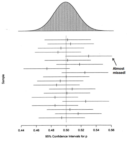
Figure 8.2. The results of a computer simulation of 20 samples of size n = 1000. We assumed that the true value of p = 0.5. At the top is the sampling distribution of pˆ [normal, with mean p and σ =√ p(1 – p)/n]. Below are the 95% confidence intervals from each sample. On average, one out of 20 (or 5%) of these intervals will not cover the point p = 0.5.

above where the sample mean is 5.96, σ is 5, and n = 25, the resulting interval would be [5.96 – 2.576(5)/ √25, 5.96 + 2.576(5)/ √25] = [3.384, 8.536]. Compare this to the 95% interval [4.00, 7.92].

Notice that for the same standard deviation and sample size, increasing the con-fidence level increases the length of the interval and also increases the chance that such intervals generated by this prescription would contain the parameter μ. Note that in this case, if μ = 8, the 95% interval would not have contained μ but the 99% interval would. This example could have been one of the 5% of cases where a 95% confidence interval does not contain the mean but the 99% interval does. The 99% interval has to be wider because it has to capture the true mean in 4/5ths of the cases where the 99% confidence interval does not. That is why the 95% interval is con-tained within the 99% interval.

We pay a price for the higher confidence in a much wider interval. For example, by establishing an extremely wide confidence interval, we are increasingly certain that it contains μ. Thus, for example, we could say with extremely high confidence that the confidence interval for the mean age of the U.S. population is between 0 and 120 years. However, this interval would not be helpful, as we would like to have a more precise estimate of μ.

If we were willing to accept a lower confidence level such as 90%, we would obtain a value of 1.645 for C, where P(–C ≤ Z ≤ C) = 0.90. In that case, for the example we are considering the interval would be [5.96 – 1.645, 5.96 + 1.645] = [4.315, 7.505]. This is a much tighter interval that is contained within the 95% in-terval. Here we gain a tighter interval at the price of lower confidence.

Another important point to note is the gain in precision of the estimate with increase in sample size. This point can be illustrated by the narrowing of the width of the confidence interval. Let us consider the 95% confidence interval for the mean that we obtained with a sample of size 25 and an estimated mean of 5.96. Suppose we increase the sample size to 100 (a factor of 4 increase) and assume that we still get a sample mean of 5.96. The 95% interval (assuming the population standard de-viation is known to be 5) is then [5.96 – 1.96 (5/√100), 5.96 + 1.96 (5/√100)] = [5.96 – 0.98, 5.96 + 0.98] = [4.98, 6.94].

This interval is much narrower and is contained inside the previous one. The in-terval width is 6.94 – 4.98 = 1.96 as compared to 7.92 – 4.00 = 3.92. Notice this in-terval is exactly half the width of the other interval. That is, if the confidence level is left unchanged and the sample size n is increased by a factor of 4, √n is increased by a factor of 2; because the interval width is 2(1.96)/ √n, the interval width is reduced by a factor of 2. Exhibit 8.1 summarizes the critical values of the standard normal distribution for calculating confidence intervals at various levels of confidence.

If the population standard deviation is unknown and we want to estimate the mean, we must use the t distribution instead of the normal distribution. So we cal-culate the sample standard deviation S and construct the t score ( – μ)/(S/√n). Recall that this quantity has Student’s t distribution with n – 1 degrees of freedom. Note that this distribution does not depend on the unknown parameters μ and σ, but it does depend on the sample size n through the degrees of freedom. This differs from the standard normal distribution that does not depend on the sample size n.

Exhibit 8.1. Two-Sided Critical Values of the Standard Normal Distribution

For standard normal distributions, we have the following critical points for two-sided confidence intervals:

C_0.90 = 1.645

C_0.95 = 1.960

C_0.99 = 2.576

For a 95% confidence interval, we need to determine C so that P(–C ≤ t ≤ C) = 0.95. For n = 25, again assume that the sample mean is 5.96, the sample standard deviation is 5, and n = 25. Then the degrees of freedom are 24, and from the table for the t distribution we see that C = 2.064. The statement P(–C ≤ t ≤ C) = 0.95 is equivalent to P[ – C(S/√n) ≤ μ ≤ X + C(S/√n)] = 0.95. So the interval is [ – C(S/√n), X + C(S/√n)]. Using C = 2.064, S = 5, n = 25, and a sample mean of 5.96, we find [5.96 – 2.064, 5.96 + 2.064] or [3.896, 8.024]. Display 8.3 summa-rizes the procedure for calculating a 95% confidence interval for a population mean when the population variance is unknown.

You should note that the interval is wider than in the case in which we knew the variance and used the normal distribution. This result occurs because there is extra variability in the t statistic due to the fact that the random quantity s is used in place of a fixed quantity σ. Remember that the t with 24 degrees of freedom has heavier tails than the standard normal distribution; this fact is reflected in the quantity C = 2.064 in place of C = 1.96 for the standard normal distribution.

Suppose we obtained the same estimates for the sample mean  and the sample standard deviation S but the sample size was increased to 100; the interval width again would decrease by a factor of 2, because the width of the interval is 2C(S/√n) and only n is changing.

Display 8.3. A 95% Confidence Interval for a Population Mean μ When the Population Variance is Unknown

The confidence interval is given by the formula

where n is the sample size, C is the 97.5 percentile of Student’s t distribution with n – 1 degrees of freedom, and σ is the sample standard deviation.