How to Select a Simple Random Sample

HOW TO SELECT A SIMPLE RANDOM SAMPLE

Simple random sampling can be defined as sampling without replacement from a population. In Section 5.5, when we cover permutations and combinations, you will learn that there are C(N, n) = N!/[(N – n)! n!] distinct samples of size n out of a pop-ulation of size N, where n! is factorial notation and stands for the product n(n – 1) (n – 2) . . . 3 2 1. The notation C(N, n) is just a symbol for the number of ways of se-lecting a subgroup of size n out of a larger group of size N, where the order of selecting the elements is not considered.

Simple random sampling has the property that each of these C(N, n) samples has the same probability of selection. One way, but not a common way, to generate a simple random sample is to order these samples from 1 all the way to C(N, n) and then randomly generate (using a uniform random number generator, which will be described shortly) an integer between 1 and C(N, n). You then choose the sample that corresponds to a chosen index.

Let us illustrate this method of generating a simple random sample with the fol-lowing example. We have six patients whom we have labeled alphabetically. So the population of patients is the set {A, B, C, D, E, F}. Suppose that we want our sam-ple size to be four. The number of possible samples will be C(6, 4) = 6!/[4! 2!] = 6 × 5 × 4 × 3 × 2 × 1/[(4 × 3 × 2 × 1)(2 × 1)]; after reducing the fraction, we obtain 3 × 5 = 15 possible samples.

We enumerate the samples as follows:

1. {A, B, C, D}

2. {A, B, C, E}

3. {A, B, C, F}

4. {A, B, D, E}

5. {A, B, D, F}

6. {A, B, E, F}

7. {A, C, D, E}

8. {A, C, D, F}

9. {A, C, E, F}

10. {A, D, E, F}

11. {B, C, D, E}

12. {B, C, D, F}

13. {B, C, E, F}

14. {B, D, E, F}

15. {C, D, E, F}.

We then use a table of uniform random numbers or a computerized pseudoran-dom number generator. A pseudorandom number generator is a computer algo-rithm that generates a sequence of numbers that behave like uniform random numbers.

Uniform random numbers and their associated uniform probability distribution will be explained in Chapter 5. To assign a random index, we take the interval [0, 1] and divide it into 15 equal parts that do not overlap. This means that the first inter-val will be from 0 to 1/15, the second from 1/15 to 2/15, and so on. A decimal approximation to 1/15 is 0.0667. So the assigned index (we will call it an index rule) depends on the uniform random number U as follows:

If 0 ≤ U < 0.0667, then the index is 1.

If 0.0667 ≤ U < 0.1333, then the index is 2.

If 0.1333 ≤ U < 0.2000, then the index is 3.

If 0.2000 ≤ U < 0.2667, then the index is 4.

If 0.2667 ≤ U < 0.3333, then the index is 5.

If 0.3333 ≤ U < 0.4000, then the index is 6.

If 0.4000 ≤ U < 0.4667, then the index is 7.

If 0.4667 ≤ U < 0.5333, then the index is 8.

If 0.5333 ≤ U < 0.6000, then the index is 9.

If 0.6000 ≤ U < 0.6667, then the index is 10.

If 0.6667 ≤ U < 0.7333, then the index is 11.

If 0.7333 ≤ U < 0.8000, then the index is 12.

If 0.8000 ≤ U < 0.8667, then the index is 13.

If 0.8667 ≤ U < 0.9333, then the index is 14.

If 0.9333 ≤ U < 1.0, then the index is 15.

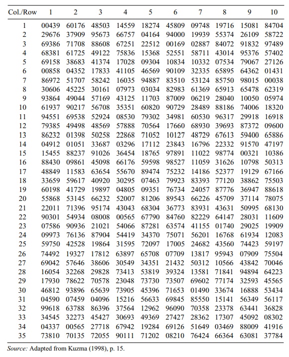
Now suppose that we consulted a table of uniform random numbers, (refer to Table 2.1). We see that this table consists of five-digit numbers. Let us arbitrarily select the number in column 7, row 19. We see that this number is 24057.

To convert 24057 to a number between 0 and 1, we simply place a decimal point in front of the first digit. Our uniform random number is then 0.24057. From the in-dex rule described previously, we see that U = 0.24057. Since 0.2000 ≤ U < 0.2667, the index is 4. We now refer back to our enumeration of samples and see that the index 4 corresponds to the sample {A, B, D, E}. So patients A, B, D, and E are selected as our sample of four patients from the set of six patients.

A more common way to generate a simple random sample is to choose four ran-dom numbers to select individual patients. This procedure is accomplished by sam-pling without replacement. First we order the patients as follows:

1. A

2. B

3. C

4. D

5. E

6. F

TABLE 2.1. Five Digit Uniform Random Numbers (350)

Then we divide [0, 1] into six equal intervals to assign the index. We choose a uniform random number U and assign the indices as follows:

If 0 ≤ U < 0.1667, then the index is 1.

If 0.1667 ≤ U < 0.3333, then the index is 2.

If 0.3333 ≤ U < 0.5000, then the index is 3.

If 0.5000 ≤ U < 0.6667, then the index is 4.

If 0.6667 ≤ U < 0.8333, then the index is 5

If 0.8333 ≤ U < 1.0, then the index is 6.

Refer back to Table 2.1. We will use the first four numbers in column 1 as our set of uniform random numbers for this sample. The resulting numbers are 00439, 29676, 69386, and 68381. For the first patient we have the uniform random number (U) 0.00439. Since 0 ≤ U < 0.1667, the index is 1. Hence, our first selection is patient A.

Now we select the second patient at random but without replacement. Therefore, A must be removed. We are left with only five indices. So we must revise our scheme. The patient order is now as follows:

1. B

2. C

3. D

4. E

5. F

The uniform random number must be divided into five equal parts, so the index assignment is as follows:

If 0 ≤ U < 0.2000, then the index is 1.

If 0.2000 ≤ U < 0.4000, then the index is 2.

If 0.4000 ≤ U < 0.6000, then the index is 3.

If 0.6000 ≤ U < 0.8000, then the index is 4.

If 0.8000 ≤ U < 1.0, then the index is 5.

The second uniform number is 29676, so our uniform number U in [0, 1] is 0.29676. Since 0.2000 ≤ U < 0.4000, the index is 2. We see that the index 2 corre-sponds to patient C.

We continue to sample without replacement. Now we have only four indices left, which are assigned as follows:

1. B

2. D

3. E

4. F

The interval from [0, 1] must be divided into four equal parts with U assigned as follows:

If 0 ≤ U < 0.2500, then the index is 1.

If 0.2500 ≤ U < 0.5000, then the index is 2.

If 0.5000 ≤ U < 0.7500, then the index is 3.

If 0.7500 ≤ U < 1.0, then the index is 4.

Since our third uniform number is 69386, U = 0.69386. Since 0.5000 ≤ U < 0.7500, the index is 3. We see that the index 3 corresponds to patient E.

We have one more patient to select and are left with only three patients to choose from. The new ordering of patients is as follows:

1. B

2. D

3. F

We now divide [0, 1] into three equal intervals as follows:

If 0 ≤ U < 0.3333, then the index is 1.

If 0.3333 ≤ U < 0.6667, then the index is 2.

If 0.6667 ≤ U < 1.0, then the index is 3.

The final uniform number is 68381. Therefore, U = 0.68381.

From the assignment above, we see that index 3 is selected and corresponds to patient F. The four patients selected are A, C, E, and F. The foregoing approach, in which patients are selected at random without replacement, is another legitimate way to generate a random sample of size 4 from a population of size 6. (When we do bootstrap sampling, which requires sampling with replacement, the methodolo-gy will be simpler than the foregoing approach.)

The second approach was simpler, in one respect, than the first approach. We did not have to identify and order all 15 possible samples of size 4. When the popula-tion size is larger than in the given example, the number of possible samples can be-come extremely large, making it difficult and time-consuming to enumerate them.

On the other hand, the first approach required the generation of only a single uni-form random number, whereas the second approach required the generation of four. However, we have large tables and fast pseudorandom number generator algo-rithms at our disposal. So generating four times as many random numbers is not a serious problem.

It may not seem obvious that the two methods are equivalent. The equivalence can be proved mathematically by using probability methods. The proof of this equivalence is beyond the scope of this text. The sampling without replacement ap-proach is not ideal because each time we select a patient we have to revise our index schemes, both the mapping of patients to indices and the choice of the index based on the uniform random number.

The use of a rejection-sampling scheme can speed up the process of sample se-lection considerably. In rejection sampling, we reject a uniform random number if it corresponds to an index that we have already picked. In this way, we can begin with the original indexing scheme and not change it. The trade-off is that we may need to generate a few more uniform random numbers in order to complete the sample. Be-cause random number generation is fast, this trade-off is worthwhile.

Let us illustrate a rejection-sampling scheme with the same set of six patients as before, again selecting a random sample of size 4. This time, we will start in the second row, first column and move across the row. Our indexing schemes are fixed as described in the next paragraphs.

First we order the patients as follows:

1. A

2. B

3. C

4. D

5. E

6. F

Then we divide [0, 1] into six equal intervals to assign the index. We choose a uniform random number U and assign the indices as follows:

If 0 ≤ U < 0.1667, then the index is 1.

If 0.1667 ≤ U < 0.3333, then the index is 2.

If 0.3333 ≤ U < 0.5000, then the index is 3.

If 0.5000 ≤ U < 0.6667, then the index is 4.

If 0.6667 ≤ U < 0.8333, then the index is 5

If 0.8333 ≤ U < 1.0, then the index is 6.

The first uniform number is 29676, so U = 0.29676. The index is 2, and the cor-responding patient is B. Our second uniform number is 37909, so U = 0.37909. The index is 3, and the corresponding patient is C. Our third uniform number is 95673, so U = 0.95673. The index is 6, and this corresponds to patient F. The fourth uni-form number is 66757, so U = 0.6676 and the index is 5; this corresponds to patient E.

Through the foregoing process we have selected patients B, C, E, and F for our sample. Thus, we see that this approach was much faster than previous approaches. We were somewhat lucky in that no index repeated; thus, we did not have to reject any samples. Usually one or more samples will be rejected due to repetition.

To show what happens when we have repeated index numbers, suppose we had started in column 1 and simply gone down the column as we did when we used the sampling without replacement approach. The first random number is 00439, corre-sponding to U = 0.00439. The resulting index is 1, corresponding to patient A. The second random number is 29676, corresponding to U = 0.29676. The resulting in-dex is 2, corresponding to patient B. The third random number is 69386, corre-sponding to U = 0.69386. The resulting index is 5, corresponding to patient E. The fourth random number is 68381, corresponding to U = 0.68381.

Again this process yields index 5 and corresponds to patient E. Since we cannot repeat patient E, we reject this number and proceed to the next uniform random number in our sequence. The number turns out to be 69158, corresponding to U = 0.69158, and index 5 is repeated again. So this number must be rejected also. The next random number is 00858, corresponding to U = 0.00858, and an index of 1, corresponding to patient A.

Now patient A already has been selected, so again we must reject the number and continue. The next uniform random number is 86972, corresponding to U = 0.86972; this corresponds to the index 6 and patient F. Because patient F has not been selected already, we accept this number and have completed the sample.

Recall the random number sequence 00439 → patient A, 29676 → patient B, 69386 → patient E, 68381 → patient E (repeat, so reject), 69158 → patient E (re-peat, so reject), 00858 → patient A (repeat, so reject), and 86972 → patient F. Because we now have a sample of four patients, we are finished. The random sample is A, B, E, and F.

We have illustrated three methods for generating simple random samples and re-peated the rejection method with a second sequence of uniform random numbers. Although the procedures are quite different from one another, it can be shown mathematically that samples generated by any of these three methods have the properties of simple random samples.

This result is important for you to remember, even though we are not showing you the mathematical proof. In our examples, the samples turned out to be different from one another. The first method led to A, B, D, E, the second to A, C, E, F, and the third to B, C, E, F, using the first sequence; and A, B, E, F when using the second sequence.

Differences occurred because of differences in the methods and differences in the sequence of uniform random numbers. But note also that even when different methods are used or different uniform random number sequences are used, it is possible to repeat a particular random sample.

Once the sample has been selected, we generally are interested in a characteristic of the patient population that we estimate from the sample. In our example, let us suppose that age is the characteristic of the population and that the six patients in the population have the following ages:

A. 26 years old

B. 17 years old

C. 45 years old

D. 70 years old

E. 32 years old

F. 9 years old

Although we generally refer to the sample as the set of patients, often the value of their characteristic is referred to as the sample. Because two patients can have the same age, it is possible to obtain repeat values in a simple random sample. The point to remember is that the individual patients selected cannot be repeated but the value of their characteristic may be repeated if it is the same for another patient.

A population parameter of interest might be the average age of the patients in the population. Because our population consists of only six patients, it is easy for us to calculate the population parameter in this instance. The mean age is defined as the sum of the ages divided by the number of patients. In this case, the population mean μ = (26 + 17 + 45 + 70 + 32 + 9)/6 = 199/6 = 33.1667.

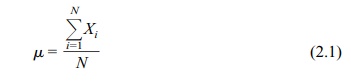
where X_i is the value for patient i and N is the population size.

Recall that a simple random sample has the property that the sample mean is an unbiased estimate of the population mean. This does not imply that the sample mean equals the population mean. It means only that the average of the sample means taken over all possible simple random samples equals the population mean.

This is a desirable statistical property and is one of the reasons why simple random sampling is used. Consider the population of six ages given previously. Suppose we choose a random sample of size 4. Suppose that the sample consists of patients B, C, E, and F. Then the sample mean  = (17 + 45 + 32 + 9)/4 = 19.5.

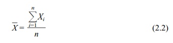
where X_i is the value for patient i in the sample and n is the sample size.

Now let us look at the four random samples that we generated previously and calculate the mean age in each case. In the first case, we chose A, B, D, E with ages 26, 17, 70, and 32, respectively. The sample mean  = (26 + 17 + 70 + 32)/4 (the sum of the ages of the sample patients divided by the total sample size). In this case  = 36.2500, which is slightly higher than the population mean of 33.1667.

Now consider case 2 with patients A, C, E, and F and corresponding ages 26, 45, 32, and 9. In this instance,  = (26 + 45 + 32 + 9)/4 = 28.0000, producing a sample mean that is lower than the population mean of 33.1667.

In case 3, the sample consists of patients B, C, E, and F with ages 17, 45, 32, and 9, respectively, and a corresponding sample mean,   = 25.7500. In case 4, the sample consists of patients A, B, E, and F with ages 26, 17, 32, and 9, respectively, and a corresponding sample mean,  = 21.0000. Thus, we see that the sample means from samples selected from the same population can differ substantially. However, the unbiasedness property still holds and has nothing to do with the variability.

What is the unbiasedness property and how do we demonstrate it? For simple random sampling, each of the C(N, n) samples has a probability of 1/C(N, n) of be-ing selected. (Chapter 5 provides the necessary background to cover this point in more detail.) In our case, each of the 15 possible samples has a probability of 1/15 of being selected.

The unbiasedness property means that if we compute all 15 sample means, sum them, and divide by 15, we will obtain the population mean. The following example will verify the unbiasedness property of sample means. Recall that the 15 samples with their respective sample means are as follows:

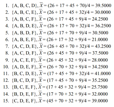
Notice that the largest mean is 43.2500, the smallest is 21.0000, and the closest to the population mean is 34.2500. The average of the 15 sample means is called the expected value of the sample mean, denoted by the symbol E.

The property of unbiasedness states that the expected value of the estimate equals the population parameter [i.e., E() = μ]. In this case, the population para-meter is the population mean, and its value is 33.1667 (rounded to four decimal places).

To calculate the expected value of the sample mean, we average the 15 values of sample means (computed previously). The average yields E() = (39.5 + 30.0 + 24.25 + 36.25 + 30.5 + 21.0 + 43.25 + 37.5 + 28.0 + 34.25 + 41.0 + 35.25 + 25.75 + 32.0 + 39.0)/15 = 497.5/15 = 33.1667. Consequently, we have demonstrated the un-biasedness property in this case. As we have mentioned previously, this statistical property of simple random samples can be proven mathematically. Sample estimates of other parameters can also be unbiased and the unbiasedness of these esti-mates for simple random samples can also be proven mathematically. But it is important to note that not all estimates of parameters are unbiased. For example, ratio estimates obtained by taking the ratio of unbiased estimates for both the numerator and denominator are biased. The interested reader may consult Cochran (1977) for a mathematical proof that the sample mean is an unbiased estimate of a finite popu-lation mean [Cochran (1977), page 22, Theorem 2.1] and the sample variance is an unbiased estimate of the finite population variance [as defined by Cochran (1977); see Theorem 2.4 ].