Exercises questions answers

EXERCISES

2.1 Why does the field of inferential statistics need to be concerned about sam-ples? Give in your own words the definitions of the following terms that per-tain to sample selection:

a.     Sample

b.     Census

c.      Parameter

d.     Statistic

e.      Representativeness

f.       Sampling frame

g.     Periodic effect

2.2 Describe the following types of sample designs, noting their similarities and differences. State also when it is appropriate to use each type of sample design.

a.     Random sample

b.     Simple random samples

c.      Convenience/grab bag samples

d.     Systematic samples

e.      Stratified

f.       Cluster

g.     Bootstrap

2.3 Explain what is meant by the term parameter estimation.

2.4 How can bias affect a sample design? Explain by using the terms selection bias, response bias, and periodic effects.

2.5 How is sampling with replacement different from sampling without replacement?

2.6 Under what circumstances is it appropriate to use rejection sampling methods?

2.7 Why would a convenience sample of college students on vacation in Fort Lauderdale, Florida, not be representative of the students at a particular col-lege or university?

2.8 What role does sample size play in the accuracy of statistical inference? Why is the method of selecting the sample even more important than the size of the sample?

Exercises 2.9 to 2.13 will help you acquire familiarity with sample selection. These exercises use data from Table 2.2.

2.9 By using the random number table (Table 2.1), draw a sample of 10 height measurements from Table 2.2. This sample is said to have size 10, or n = 10. The rows and columns in Table 2.2 have numbers, which in combination are the “addresses” of specific height measurements. For example, the number defined by row 15, column 4 denotes the 154th height measurement, or 61. 

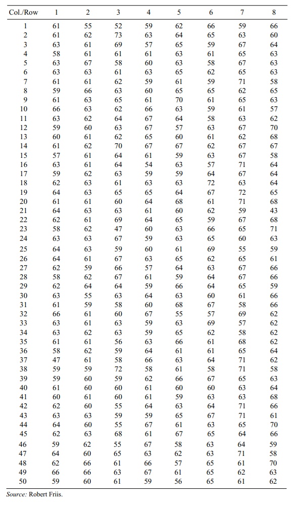
TABLE 2.2. Heights in Inches of 400 Female Clinic Patients

Use two indices based on numbers from Table 2.1. Draw one random number to select the row between 1 and 50 and another to choose the column between 1 and 8. Use the rejection method. List the ten values you have selected by this process. What name is given to the kind of sample you have selected?

2.10 Again use Table 2.2 to select a sample, but this time select only one random number from Table 2.1. Start in the row determined by the index for that ran-dom number. Choose the first value from the first column in that row; then skip the next seven columns and select the second value from column 8. Con-tinue skipping seven consecutive values before selecting the next value. When you come to the end of the row, continue the procedure on the next row. What kind of sampling procedure is this? Can bias be introduced when you sample in this way?

2.11 From the 400 height measurements in Table 2.2, we will take a sample of ten distinct values by taking the first six values in row 1 and the two values in the last two columns in row 2 and the last two columns in row 3. Let these ten values comprise the sample. Draw a sample of size 10 by sampling with re-placement from these 10 measurements.

a. List the original sample and the sample generated by sampling with re-placement from it.

b. What do we call the sample generated by sampling with replacement?

2.12 Repeat the procedure of Exercise 2.11 five times. List all five samples. How do they differ from the original sample?

2.13 Describe the population and the sample for:

a. Exercise 2.9

b. The bootstrap sampling plan in Exercise 2.11

2.14 Suppose you selected a sample from Table 2.2 by starting with the number in row 1, column 2. You then proceed across the row, skipping the next five numbers and take the sixth number. You continue in this way, skipping five numbers and taking the sixth, going to the leftmost element in the next row when all the elements in a row are exhausted, until you have exhausted the table.

a. What is such a sample selection scheme called?

b. Could any possible sources of bias arise from using this scheme?

Answer:

2.9 From Table 2.1, start in the first column and the third row and proceed across the row to generate the random numbers, going back to the first column on the next row when a row is completed. Placing a zero and a decimal point in front of the first digit of the number (we will do this throughout), we get for the first random number 0.69386. This random number picks the row. We multiply 0.69386 by 50, getting 34.693. We will always round up. This will give us integers between 1 and 50. So we take row 35. Now the next number in the table is used for the column. It is 0.71708. Since there are 8 columns, we multiply 0.71708 by 8 to get 5.7366 and round up to get 6. Now, the first sample from the table is (35, 6), the value in row 35 column 6. We look this up in Table 2.2 and find the height to be 61 inches.

For the second measurement, we take the next pair of numbers, 0.88608 and 0.67251. After the respective multiplications we have row 45 and column 6. We compare (45, 6) to our list, which consists only of (35, 6). Since this pair does not repeat a pair on the list, we accept it. The list is now (35, 6) and (45, 6) and the sam-ples are, respectively, 61 and 65.

For the third measurement the next pair of random numbers is 0.22512 and 0.00169, giving the pair (12, 1). Since this pair is not on the list, we accept and the list becomes (35, 6), (45, 6), and (12, 1), with corresponding measurements 61, 65, and 59.

The next pair is 0.02887 and 0.84072, giving the pair (2, 7). This is accepted since it does not appear on the list. The resulting measurement is 63.

The next pair is 0.91832 and 0.97489 giving the pair (46, 8). Again, we accept. The corresponding measurement is 59.

We are half way to the result. The list of pairs is (35, 6), (45, 6), (12, 1), (2, 7), and (46, 8), corresponding to the sample measurements 61, 65, 59, 63, and 59.

The next pair of random numbers is 0.68381 and 0.61725 (note at this point we had to move to row 4 column 1). The pair is (35, 5). This again is not on the list and the corresponding measurement is 66.

The next pair of random numbers is 0.49122 and 0.75836 corresponding to the pair (25, 7). This is not on the list so we accept it and the corresponding sample measurement is 55.

The next pair of random numbers is 0.58711 and 0.52551 corresponding to the pair (8, 5). This pair is again not on our list so we accept it. The sample measure-ment is 65.

The next pair of random numbers is 0.58711 and 0.43014, corresponding to the pair (30, 4). This pair is again not on our list so we accept it. The sample measure-ment is 64.

The next pair of random numbers is 0.95376 and 0.57402, corresponding to the pair (48, 5). This pair is again not on our list so we accept it. The sample measurement is 57.

We now have 10 samples. Since we only took 10 out of 400 numbers (50 rows by 8 columns), our chances of a rejection on any sample was small and we did not get one.

The resulting 10 pairs are (35, 6), (45, 6), (12, 1), (2,7), (46,8), (35, 5), (25,7), (8, 5), (30, 4) and (48, 5) and the corresponding sample of ten measurements is 61, 65, 59, 63, 59, 66, 55, 65, 64, and 57.

Despite the complicated mechanism we used to generate the sample, this consti-tutes what we call a simple random sample since each of the 400 samples has prob-ability 1/400 of being selected first and each of the remaining 399 has probability 1/399 of being selected second, given they weren’t chosen first, etc.

2.11 a. The original sample is 61, 55, 52, 59, 62, 66, 63, 60, 67, and 64. We then index these samples 1–10. Index 1 corresponds to 61, 2 to 55, 3 to 52, 4 to 59, 5 to 62, 6 to 66, 7 to 63, 8 to 60, 9 to 67, and 10 to 64. We use a table of random num-bers to pick the index. We will do this by running across row 21 of Table 2.1 to gen-erate the 10 indices. The random numbers on row 21 are:

22011                   71396                   95174                   43043                   68304              36773              83931                   43631                   50995        68130

This we interpret as 0.22011, 0.71396, 0.95174, 0.43043, 0.68304, 0.36773, 0.83931, 0.43631, 0.50995, and 0.68130. To get the index, we multiply these num-bers by 10 and round up to the next integer. The resulting indices are, respectively, 3, 8, 10, 5, 7, 4, 9, 5, 6, and 7. We see that indices 5 and 7 each repeated once and indices 1 and 2 did not occur. The corresponding sample is 52, 60, 64, 62, 63, 59, 67, 62, 66, and 63.

b. The name we give to sampling with replacement n times from a sample of size n is bootstrap sampling. The sample we obtained we call a bootstrap sample.

2.13 a. A population is a complete list of all the subjects you are interested in. For Exercise 2.9, it consisted of the 400 height measurements for the female clinic pa-tients. The sample is the chosen subset of the population, often selected at random. In this case it consisted of a random sample of 10 measurements corresponding to the female patients in specific rows and columns of the table. The resulting 10 pairs were (35, 6), (45, 6), (12, 1), (2,7), (46,8), (35, 5), (25,7), (8, 5), (30, 4), and (48, 5) and the corresponding sample of 10 measurements were 61, 65, 59, 63, 59, 66, 55, 65, 64, and 57.

b. For the bootstrap sampling plan in Exercise 2.11, the population is the same set of 400 height measurements in Table 2.2. The original sample is a subset of size 10 taken from this population in a systematic fashion, as described in Exercise 2.11. The bootstrap sample is then obtained by sampling with replacement from this original sample of size 10. The resulting bootstrap sample is a sample of size 10 that may have some of the original sample values repeated one or more times depending on the result of the random drawing. As shown in our solution, the indices 5 and 7 repeated once each.

2.14 a. This method of sampling is systematic sampling. It specifically is a periodic method.

b. Because of the cyclic nature of the sampling scheme, there is a danger of bias. If the data is also cyclic with the same period we could be sampling only the peak values (or only the trough values). In that case, the sample estimate of the mean would be biased on the high side if we sampled the peaks and on the low side if we sampled the troughs.