Measures of Central Tendency

Summary Statistics

MEASURES OF CENTRAL TENDENCY

The previous chapter, which discussed data displays such as frequency histograms and frequency polygons, introduced the concept of the shape of distributions of data. For example, a frequency polygon illustrated the distribution of body mass in-dex data. Chapter 4 will expand on these concepts by defining measures of central tendency and measures of dispersion.

Measures of central tendency are numbers that tell us where the majority of values in the distribution are located. Also, we may consider these measures to be the center of the probability distribution from which the data were sampled. An example is the average age in a distribution of patients’ ages. Section 4.1 will cover the following measures of central tendency: arithmetic mean, median, mode, geometric mean, and harmonic mean. These measures also are called measures of location. In contrast to measures of central tendency, measures of dispersion inform us about the spread of values in a distribution. Section 4.2 will present measures of dispersion

1. The Arithmetic Mean

The arithmetic mean is the sum of the individual values in a data set divided by the number of values in the data set. We can compute a mean of both a finite population and a sample. For the mean of a finite population (denoted by the symbol μ), we sum the individual observations in the entire population and divide by the popula-tion size, N. When data are based on a sample, to calculate the sample mean (denoted by the symbol () we sum the individual observations in the sample and divide by the number of elements in the sample, n. The sample mean is the sample analog to the mean of a finite population. Formulas for the population (4.1a) and sample means (4.1b) are shown below; also see Table 4.1.

TABLE 4.1. Calculation of Mean (Small Population, N = 5)

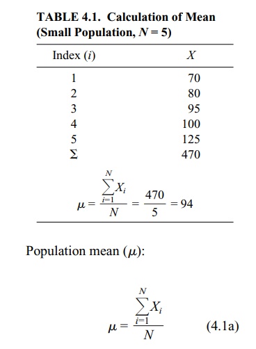
where X_i are the individual values from a finite population of size N.

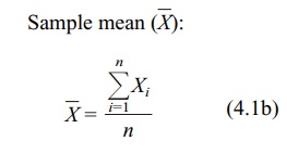
where X_i are the individual values of a sample of size n.

The population mean (and also the population variance and standard deviation) is a parameter of a distribution. Means, variances, and standard deviations of finite populations are almost identical to their sample analogs. You will learn more about these terms and appreciate their meaning for infinite populations after we cover absolutely continuous distributions and random variables in Chapter 5. We will refer to the individual values in the data set as elements, a point that will be discussed in more detail in Chapter 5, which covers probability theory.

Statisticians generally use the arithmetic mean as a measure of central tendency for numbers that are from a ratio scale (e.g., many biological values, height, blood sugar, cholesterol), from an interval scale (e.g., Fahrenheit temperature or personal-ity measures such as depression), or from an ordinal scale (high, medium, low). The values may be either discrete or continuous; for example, ranking on an attitude scale (discrete values) or blood cholesterol measurements (continuous).

It is important to distinguish between a continuous scale such as blood cholesterol and cholesterol measurements. While the scale is continuous, the measurements we record are discrete values. For example, when we record a cholesterol measurement of 200, we have converted a continuous variable into a discrete measurement. The speed of an automobile is also a continuous variable. As soon as we state a specific speed, for example, 60 miles or 100 kilometers per hour, we have created a discrete measurement. This example becomes clearer if we have a speedometer that gives a digital readout such as 60 miles per hour.

For large data sets (e.g., more than about 20 observations when performing calculations by hand), summing the individual numbers may be impractical, so we use grouped data. When using a computer, the number of values is not an issue at all. The procedure for calculating a mean is somewhat more involved for grouped data than for ungrouped data. First, the data need to be placed in a frequency table, as illustrated in Chapter 3. We then apply Formula 4.2, which specifies that the midpoint of each class interval (X) is multiplied by the frequency of observation in that class.

The mean using grouped data is

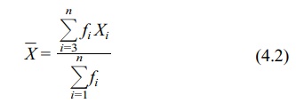
where X_i is the midpoint of the ith interval and f_i is the frequency of observations in the ith interval.

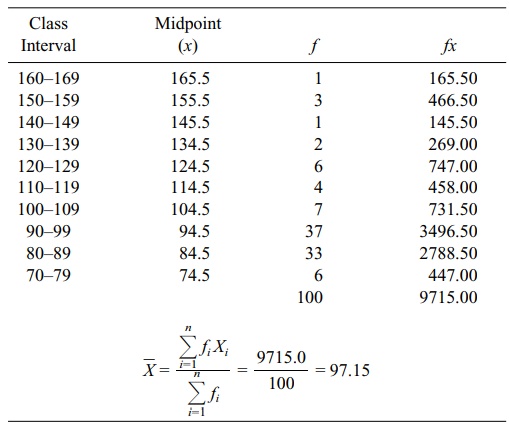
In order to perform the calculation specified by Formula 4.2, first we need to place the data from Table 4.2 in a frequency table, as shown in Table 4.3. For a re-view of how to construct such a table, consult Chapter 3. From Table 4.3, we can see that ΣfX = 9715, Σf = n = 100, and that the mean is estimated as 97.2 (rounding to the nearest tenth).

2. The Median

Previously in Chapter 3, we defined the term median and illustrated its calculation for small data sets. In review, the median refers to the 50% point in a frequency distribution of a population. 

TABLE 4.2. Plasma Glucose Values (mg/dl) for a Sample of 100 Adults, Aged 20–74 Years

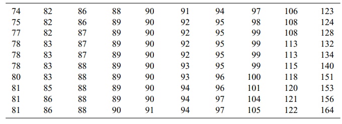
TABLE 4.3. Calculation of a Mean from a Frequency Table (Using Data from Table 4.2)

When data are grouped in a frequency table, the median is an estimate because we are unable to calculate it precisely. Thus, Formula 4.3 is used to estimate the median from data in a frequency table:

median = lower limit of the interval + i(0.50n – cf)                             (4.3)

where i = the width of the interval

n = sample size (or N = population size)

cf = the cumulative frequency below the interval that contains the median

The sample median (an analog to the population median) is defined in the same way as a population median. For a sample, 50% of the observations fall below and 50% fall above the median. For a population, 50% of the probability distribution is above and 50% is below the median.

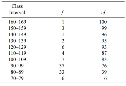
In Table 4.4, the lower end of the distribution begins with the class 70–79. The column “cf” refers to the cumulative frequency of cases at and below a particular interval. For example, the cf at interval 80–89 is 39. The cf is found by adding the numbers in columns f and cf diagonally; e.g., 6 + 33 = 39. First, we must find the interval in which the median is located. There are a total of 100 cases, so one-half of them (0.50n) equals 50. By inspecting the cumulative frequency column, we find the interval in which 50% of the cases (the 50th case) fall in or below: 90–99. The lower real limit of the interval is 89.5.

Here is a point that requires discussion. Previously, we stated that the measurements from a continuous scale represent discrete values. 

TABLE 4.4. Determining a Median from a Frequency Table

The numbers placed in the frequency table were continuous numbers rounded off to the nearest unit. The real limits of the class interval are halfway between adjacent intervals. As a result, the real limits of a class interval, e.g., 90–99, are 89.5 to 99.5. The width of the interval (i) is (99.5 – 89.5), or 10. Thus, placing these values in Formula 4.3 yields

median = 89.5 + 10[(0.50)(100) – 39] = 97.47

For data that have not been grouped, the sample median also can be calculated in a reasonable amount of time on a computer. The computer orders the observations from smallest to largest and finds the middle value for the median if the sample size is odd. For an even number of observations, the sample does not have a middle value; by convention, the sample median is defined as the average of two values that fall in the middle of a distribution. The first number in the average is the largest ob-servation below the halfway point and the second is the smallest observation above the halfway point.

Let us illustrate this definition of the median with small data sets. Although the definition applies equally to a finite population, assume we have selected a small sample. For n = 7, the data are {2.2, 1.7, 4.5, 6.2, 1.8, 5.5, 3.3}. Ordering the data from smallest to largest, we obtain {1.7, 1.8, 2.2, 3.3, 4.5, 5.5, 6.2}. The middle observation (median) is the fourth number in the sequence; three values fall below 3.3 and three values fall above 3.3. In this case, the median is 3.3.

Suppose n = 8 (the previous data set plus one more observation, 5.7). The new data set becomes {1.7, 1.8, 2.2, 3.3, 4.5, 5.5, 5.7, 6.2}. When n is even, we take the average of the two middle numbers in the data set, e.g., 3.3 and 4.5. In our example, the sample median is (3.3 + 4.5)/2 = 3.9. Note that there are three observations above and three below the two middle observations.

3. The Mode

The mode refers to the class (or midpoint of the class) that contains the highest fre-quency of cases. In Table 4.4, the modal class is 90–99. When a distribution is por-trayed graphically, the mode is the peak in the graph. Many distributions are multi-modal, referring to the fact that they may have two or more peaks. Such multimodal distributions are of interest to epidemiologists because they may indicate different causal mechanisms for biological phenomena, for example, bimodal distributions in the age of onset of diseases such as tuberculosis, Hodgkins disease, and meningo-coccal disease. Figure 4.1 illustrates unimodal and bimodal distributions.

4. The Geometric Mean

The geometric mean (GM) is found by multiplying a set of values and then finding their nth root. All of the values must be non-0 and greater than 1. Formula 4.4 shows how to calculate a GM.

A GM is preferred to an arithmetic mean when several values in a data set are much higher than all of the others. These higher values would tend to inflate or dis-tort an arithmetic mean. For example, suppose we have the following numbers: 10, 15, 5, 8, 17. The arithmetic mean is 11. Now suppose we add one more number- 100—to the previous five numbers. Then the arithmetic mean is 25.8, an inflated value not very close to 11. However, the geometric mean is 14.7, a value that is closer to 11.

In practice, is it desirable to use a geometric mean? When greatly differing val-ues within a data set occur, as in some biomedical applications, the geometric mean becomes appropriate. To illustrate, a common use for the geometric mean is to de-termine whether fecal coliform levels exceed a safe standard. (Fecal coliform bacte-ria are used as an indicator of water pollution and unsafe swimming conditions at

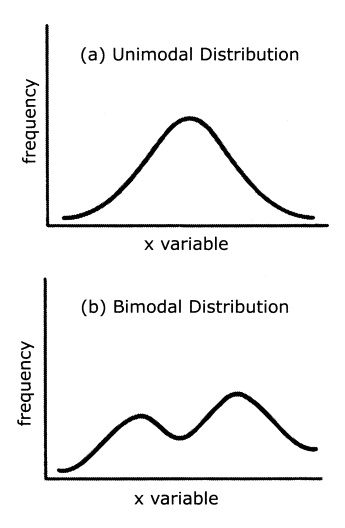
Figure 4.1. Unimodal and bimodal distribution curves. (Source: Authors.)

beaches.) For example, the standard may be set at a 30-day geometric mean of 200 fecal coliform units per 100 ml of water. When the water actually is tested, most of the individual tests may fall below 200 units. However, on a few days some of the values could be as high as 10,000 units. Consequently, the arithmetic mean would be distorted by these extreme values. By using the geometric mean, one obtains an average that is closer to the average of the lower values. To cite another example, when the sample data do not conform to a normal distribution, the geometric mean is especially useful. A log transformation of the data will produce a symmetric dis-tribution that is normally distributed.

Review Formula 4.4 and note the nth root of the product of a set of numbers. You may wonder how to find the nth root of a number. This problem is solved by logarithms or, much more easily, by using the “geometric mean function” in a spreadsheet program.

Here is a simple calculation example of the GM. Let X₁, X₂, X₃, . . . , X_n denote our sample of n values. The geometric mean is the nth root of the product of these values, or (X₁ X₂ X₃ . . . X_n)^1/n .

If we apply the log transformation to this geometric mean we obtain {log(X₁) + log(X₂) + log(X₃) + . . . + log(X_n)}/n. From these calculations, we see that the GM is the arithmetic mean of the data after transforming them to a log scale. On the log scale, the data become symmetric. Consequently, the arithmetic mean is the natural parameter to use for the location of the distribution, confirming our suspicion that the geometric mean is the correct measure of central tendency on the original scale.

5. The Harmonic Mean

The harmonic mean (HM) is the final measure of location covered in this chapter. Although the HM is not used commonly, we mention it here because you may en-counter it in the biomedical literature. Refer to Iman (1983) for more information about the HM, including applications and relationships with other measures of loca-tion, as well as additional references.

The HM is the reciprocal of the arithmetic average of the reciprocals of the orig-inal observations. Mathematically, we define the HM as follows: Let the original observations be denoted by X₁, X₂, X₃, . . . , X_n. Consider the observations Y₁, Y₂, Y₃, . . . , Y_n obtained by reciprocal transformation, namely Y_i = 1/X_i for i = 1, 2, 3, . . . , n. Let Y_h denote the arithmetic average of the Y’s, where

The harmonic mean (HM) of the X’s is 1/Y_h:

where Y_i = 1/X_i for i = 1, 2, 3, . . . , n and Y_h = (ΣY_i)/n.

6. Which Measure Should You Use?

Each of the measures of central tendency has strengths and weaknesses. The mode is difficult to use when a distribution has more than one mode, especially when these modes have the same frequencies. In addition, the mode is influenced by the choice of the number and size of intervals used to make a frequency distribution.

The median is useful in describing a distribution that has extreme values at either end; common examples occur in distributions of income and selling prices of houses. Because a few extreme values at the upper end will inflate the mean, the median will give a better picture of central tendency.

Finally, the mean often is more useful for statistical inference than either the mode or the median. For example, we will see that the mean is useful in calculating an important measure of variability: variance. The mean is also the value that mini-mizes the sum of squared deviations (mean squared error) between the mean and the values in the data set, a point that will be discussed in later chapters (e.g., Chapter 12) and that is exceedingly valuable for statistical inference.

The choice of a particular measure of central tendency depends on the shape of the population distribution. When we are dealing with sample-based data, the distri-bution of the data from the sample may suggest the shape of the population distrib-ution. For normally distributed data, mathematical theory of the normal distribution (to be discussed in Chapter 6) suggests that the arithmetic mean is the most appro-priate measure of central tendency. Finally, as we have discussed previously, if a log transformation creates normally distributed data, then the geometric mean is ap-propriate to the raw data.

How are the mean, median, and mode interrelated? For symmetric distributions, the mean and median are equal. If the distribution is symmetric and has only one mode, all three measures are the same, an example being the normal distribution. For skewed distributions, with a single mode, the three measures differ. (Refer to Figure 4.2.) For positively skewed distributions (where the upper, or left, tail of the distribution is longer (“fatter”) than the lower, or right, tail) the measures are ordered as follows: mode < median < mean. For negatively skewed distributions (where the lower tail of the distribution is longer than the upper tail), the reverse or-dering occurs: mean < median < mode. 

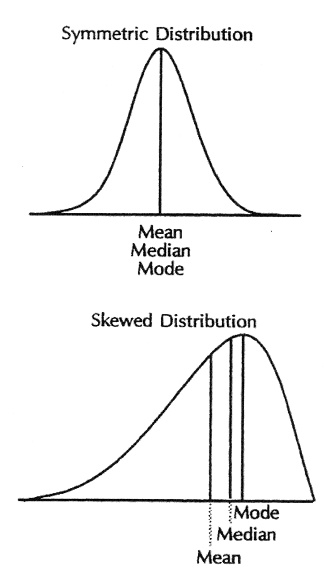
Figure 4.2. Mean, median, and mode, symmetric and skewed distributions. (Source: Centers for Dis-ease Control and Prevention (1992). Principles of Epidemiology, 2nd Edition, Figure 3.11.)

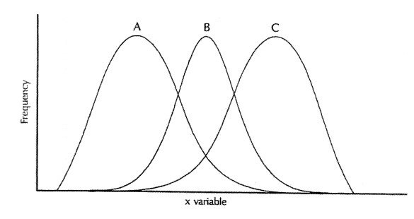
Figure 4.3. Symmetric (B) and skewed distributions: right skewed (A) and left skewed (C). (Source: Centers for Disease Control and Prevention (1992). Principles of Epidemiology, 2nd Edition, Figure 3.5)

Figure 4.3 shows symmetric and skewed distributions. The fact that the median is closer to the mean than is the mode led Karl Pearson to observe that for moderately skewed distributions such as the gamma distribution, mode – mean ≈ 3(median – mean). See Stuart and Ord (1994) and Kotz and Johnson (1985) for more details on these relationships.