Probability Rules

PROBABILITY RULES

Product (Multiplication) Rule for Independent Events

If A and B are independent events, their joint probability of occurrence is given by the Formula 5.1:

P(A ∩ B) = P(A) × P(B)                                   (5.1)

For a clear application of this rule, consider the experiment in which we roll two dice. What is the probability of a 1 on the first roll and a 2 or 4 on the second roll?

First of all, the outcome on the first roll is independent of the outcome on the second roll; therefore, define A = {get a 1 on one die and any outcome on the sec-ond die}, and let B = {any outcome on one die and a 2 or a 4 on the second die}. We can describe A as the following set of elementary events: A = [{1, 1}, {1, 2}, {1, 3}, {1, 4}, {1, 5}, {1, 6}] and B = [{1, 2}, {1, 4}, {2, 2}, {2, 4}, {3, 2}, {3, 4}, {4, 2}, {4, 4}, {5, 2}, {5, 4}, {6, 2}, {6, 4}].

The event C = A ∩ B = [{1, 2}, {1, 4}]. By the law of multiplication for inde-pendent events, P(C) = P(A) × P(B) = (1/6) × (1/3) = 1/18. You can check this by considering the elementary events associated with C. Since there are two events, each with probability 1/36, P(C) = 2/36 = 1/18.

Addition Rule for Mutually Exclusive Events

If A and B are mutually exclusive events, then the probability of their union (i.e., the probability that at least one of the events, A or B, occurs) is given by Formula 5.2. Mutually exclusive events are also called disjoint events. In terms of symbols, event A and event B are disjoint if A ∩ B = Ø.

P(AU B) = P(A) + P(B)                   (5.2)

Again, consider the example of rolling the dice; we roll two dice once. Let A be the event that both dice show the same number, which is even, and let B be the event that both dice show the same number, which is odd. Let C = A U B. Then C is the event in which the roll of the dice produces the same number, either even or odd.

For the two dice together, C occurs in six elementary ways: {1, 1}, {2, 2}, {3, 3}, {4, 4}, {5, 5}, and {6, 6}. A occurs in three elementary ways, namely, {2, 2}, {4, 4}, and {6, 6}. B also occurs in three elementary ways, namely, {1, 1}, {3, 3}, and {5, 5}.

P(C) = 6/36 = 1/6, whereas P(A) = 3/36 = 1/12 and P(B) = 3/36 = 1/12. By the addition law for mutually exclusive events, P(C) = P(A) + P(B) = (1/12) + (1/12) = 2/12 = 1/6. Thus, we see that the addition rule applies.

An application of the rule of addition is the rule for complements, shown in For-mula 5.3. Since A and A^c are mutually exclusive and complementary, we have Ω = A U A^c and P(Ω) = P(AU A^c) = P(A) + P(A^c) = 1.

P(A^c) = 1 – P(A)                         (5.3)

In general, the addition rule can be modified for events A and B that are not disjoint. Let A and B be the sets identified in the Venn diagram in Figure 5.3. Call the overlap area C = A ∩ B. Then, we can divide the set A U B into three mutually exclusive sets as labeled in the diagram, namely, A ∩ B^c, C, and B ∩ A^c.

When we compute P(A) + P(B), we obtain P(A) = P(A ∩ B) + P(A ∩ B^c) and P(B) = P(B ∩ A) + P(B ∩ A^c). Now A ∩ B = B ∩ A. So P(A) + P(B) = P(A ∩ B) + P(A ∩ B^c) + P(B∩  A) + P(B ∩ A^c) = P(A ∩ B^c) + P(B ∩ A^c) + 2P(C). But P(A U B) = P(A ∩ B^c) + P(B ∩ A^c) + P(C) because it is the union of these three mutually exclusive events.

The problem with the summation formula is that P(C) is counted twice. We remedy this error by subtracting P(C) once. This subtraction yields the generalized ad-dition formula for union of arbitrary events, shown as Formula 5.4:

P(A U B) = P(A) + P(B) – P(A ∩ B)                            (5.3)

Note that Formula 5.4 applies to mutually exclusive events A and B as well, since for mutually exclusive events, P(A ∩ B) = 0. Next we will generalize the mul-tiplication rule, but first we need to define conditional probabilities.

Suppose we have two events, A and B, and we want to define the probability of A occurring given that B will occur. We call this outcome the conditional probability of A given B and denote it by P(A|B). Definition 5.4.1 presents the formal mathe-matical definition of P(A|B).

Definition 5.4.1: Conditonal Probability of A Given B. Let A and B be arbitrary events. Then P(A|B) = P(A∩ B)/P(B).

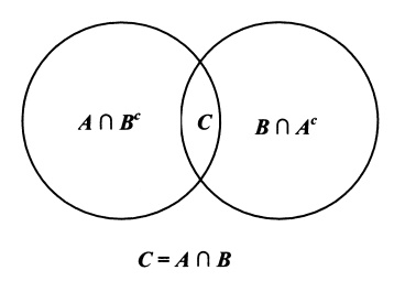
Figure 5.3. Decomposition of AU B into disjoint sets.

Consider rolling one die. Let A = {a 2 occurs} and let B = {an even number occurs}. Then A = {2} and B = [{2}, {4}, {6}]. P(A B) = 1/6 because A ∩ B = A = {2} and there is 1 chance out of 6 for 2 to come up. P(B) = 1/2 since there are 3 ways out of 6 for an even number to occur. So by definition, P(A|B) = P(A ∩ B)/P(B) = (1/6)/(1/2) = 2/6 = 1/3.

Another way to understand conditional probabilities is to consider the restricted outcomes given that B occurs. If we know that B occurs, then the outcomes {2}, {4}, and {6} are the only possible ones and they are equally likely to occur. So each outcome has the probability 1/3; hence, the probability of a 2 is 1/3. That is just what we mean by P(A|B). Directly from Definition 5.4.1, we derive Formula 5.5 for the general law of conditional probabilities:

P(A|B) = P(A ∩ B)/P(B)                                  (5.5)

Multiplying both sides of the equation by P(B), we have P(A|B) P(B) = P(A ∩ B). This equation, shown as Formula 5.6, is the generalized multiplication law for the in-tersection of arbitrary events:

P(A ∩ B) = P(A|B)P(B)                           (5.6)

The generalized multiplication formula holds for arbitrary events A and B. Conse-quently, it also holds for independent events.

Suppose now that A and B are independent; then, from Formula 5.1, P(A ∩ B) = P(A) P(B). On the other hand, from Formula 5.6, P(A ∩ B) = P(A|B) P(B). So P(A|B) P(B) = P(A) P(B).

Dividing both sides of P(A|B) P(B) = P(A) P(B) by P(B) (since P(B) > 0), we have P(A|B) = P(A). That is, if A and B are independent, then the probability of A given B is the same as the unconditional probability of A.

This result agrees with our intuitive notion of independence, namely, condition-ing on B does affect the chances of A’s occurrence. Similarly, one can show that if A and B are independent, then P(B|A) = P(B).