Probability Distributions

PROBABILITY DISTRIBUTIONS

Probability distributions describe the probability of events. Parameters are characteristics of probability distributions. The statistics that we have used to estimate pa-rameters are also called random variables. We are interested in the distributions of these statistics and will use them to make inferences about population parameters.

We will be able to draw inferences by constructing confidence intervals or test-ing hypotheses about the parameters. The methods for doing this will be developed in Chapters 8 and 9, but first you must learn the basic probability distributions and the underlying bases for the ones we will use later.

We denote the statistic, or random variable, with a capital letter—often “X.” We distinguish the random variable X from the value it takes on in a particular experi-ment by using a lower case x for the latter value. Let A = [X = x]. Assume that A = [X = x] is an event that is similar to the events described earlier in this chapter. If X is a discrete variable that takes on only a finite set of values, the events of the form A = [X = x] have positive probabilities associated with some finite set of values for x and zero probability for all other values of x.

A discrete variable is one that can take on distinct values for each individual measurement. We can assign a positive probability to each number. The probabili-ties associated with each value of a discrete variable can form an infinite set of val-ues, known as an infinite discrete set. The discrete set also could be finite. The most common example of an infinite discrete set is a Poisson random variable, which as-signs a positive probability to all the non-negative integers, including zero. The Poisson distribution is a type of distribution used to portray events that are infre-quent (such as the number of light bulb failures). The degree of occurrence of events is determined by the rate parameter. By infrequent we mean that in a short interval of time there cannot be two events occurring. An example of a distribution that is discrete and finite is the binomial distribution, to be discussed in detail later. For the binomial distribution, the random variable is the number of successes in n trials; it can take on the n + 1 discrete values 0, 1, 2, 3, . . . , n.

Frequently, we will deal with another type of random variable, the absolutely continuous random variable. This variable can take on values over a continuous range of numbers. The range could be an interval such as [0, 1], or it could be the entire set of real numbers. A random variable with a uniform distribution illustrates a distribution that uses a range of numbers in an interval such as [0, 1]. A uniform distribution is made from a dataset in which all of the values have the same chance of occurrence. The normal, or Gaussian, distribution is an example of an absolutely continuous distribution that takes on values over the entire set of real numbers.

Absolutely continuous random variables have probability densities associated with them. You will see that these densities are the analogs to probability mass functions that we will define for discrete random variables.

For absolutely continuous random variables, we will see that events such as A = P(X = x) are meaningless because for any value x, P(X = x) = 0. To obtain mean-ingful probabilities for absolutely continuous random variables, we will need to talk about the probability that X falls into an interval of values such as P(0 < X < 1). On such intervals, we can compute positive probabilities for these random variables.

Probability distributions have certain characteristics that can apply to both ab-solutely continuous and discrete distributions. One such property is symmetry. A probability distribution is symmetric if it has a central point at which we can con-struct a vertical line so that the shape of the distribution to the right of the line is the mirror image of the shape to the left.

We will encounter a number of continuous and discrete distributions that are symmetric. Examples of absolutely continuous distributions that are symmetric are the normal distribution, Student’s t distribution, the Cauchy distribution, the uni-form distribution, and the particular beta distribution that we discuss at the end of this chapter.

The binomial distribution previously mentioned (covered in detail in the next section) is a discrete distribution. The binomial distribution is symmetric if, and only if, the success probability p = 1/2. To review, the toss of a fair coin has two possible outcomes, heads or tails. If we want to obtain a head when we toss a coin, the head is called a “success.” The probability of a head is 1/2.

Probability distributions that are not symmetric are called skewed distributions. There are two kinds of skewed distributions: positively skewed and negatively skewed. Positively skewed distributions have a higher concentration of probability mass or density to the left and a long, declining tail to the right, whereas negatively skewed distributions have probability mass or density concentrated to the right with a long, declining tail to the left.

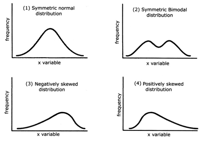
Figure 5.4. Continuous probability densities.

Figure 5.4 shows continuous probability densities corresponding to: (1) a symmetric normal distribution, (2) a symmetric bimodal distribution, (3) a negatively skewed distribution, and (4) a positively skewed distribution. The negative expo-nential distribution and the chi-square distribution are examples of positively skewed distributions.

Beta distributions and binomial distributions (both to be described in detail later) can be symmetric, positively skewed, or negatively skewed depending on the val-ues of certain parameters. For instance, the binomial distribution is positively skewed if p < 1/2, is symmetric if p = 1/2, and is negatively skewed if p > 1/2.

Now let us look at a familiar experiment and define a discrete random variable associated with that experiment. Then, using what we already know about probabil-ity, we will be able to construct the probability distribution for this random variable.

For the experiment, suppose that we are tossing a fair coin three times in indepen-dent trials. We can enumerate the elementary outcomes: a total of eight. With H de-noting heads and T tails, the triplets are: {H, H, H}, {H, H, T}, {H, T, H}, {H, T, T}, {T, H, H}, {T, H, T}, {T, T, H}, and {T, T, T}. We can classify these eight elementary events as follows: E₁ = {H, H, H}, E₂ = {H, H, T}, E₃ = {H, T, H}, E₄ = {H, T, T}, E₅ = {T, H, H}, E₆ = {T, H, T}, E₇ = {T, T, H}, and E₈ = {T, T, T}.

We want Z to denote the random variable that counts the number of heads in the experiment. By looking at the outcomes above, you can see that Z can take on the values 0, 1, 2, and 3. You also know that the 8 elementary outcomes above are equally likely because the coin is fair and the trials are independent. So each triplet has a probability of 1/8. You have learned that elementary events are mutually ex clusive (also called disjoint). Consequently, the probability of the union of elemen-tary events is just the sum of their individual probabilities.

You are now ready to compute the probability distribution for Z. Since Z can be only 0, 1, 2, or 3, we know its distribution once we compute P(Z = 0), P(Z = 1), P(Z = 2), and P(Z = 3). Each of these events {Z = 0}, {Z = 1}, {Z = 2}, and {Z = 3} can be described as the union of a certain set of these elementary events.

For example, Z = 0 only if all three tosses are tails. E₈ denotes the elementary event {T, T, T}. We see that P(Z = 0) = P(E₈) = 1/8. Similarly, Z = 3 only if all three tosses are heads. E₁ denotes the event {H, H, H}; therefore, P(Z = 3) = P(E₁) = 1/8.

Consider the event Z = 1. For Z = 1, we have exactly one head and two tails. The elementary events that lead to this outcome are E₄ = {H, T, T}, E₆ = {T, H, T}, and E₇ = {T, T, H}. So P(Z = 1) = P(E₄ U E₆ U E₇). By the addition law for mutually exclusive events, we have P(Z = 1) = P(E₄ U E₆ U E₇) = P(E₄) + P(E₆) + P(E₇) = 1/8 + 1/8 + 1/8 = 3/8.

Next, consider the event Z = 2. For Z = 2 we have exactly one tail and two heads. Again there are three elementary events that give this outcome. They are E₂ = {H, H, T}, E₃ = {H, T, H}, and E₅ = {T, H, H}. So P(Z = 2) = P(E₂ U E₃ U E₅). By the addition law for mutually exclusive events, we have P(Z = 2) = P(E₂ U E₃ U E₅) = P(E₂) + P(E₃) + P(E₅) = 1/8 + 1/8 + 1/8 = 3/8.

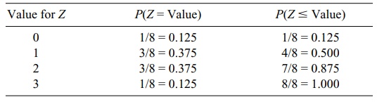
Table 5.1 gives the distribution for Z. The second column of the table is called the probability mass function for Z. The third column is the cumulative probability function. The value shown in the first cell of the third column is carried over from the first cell of the second column. The value shown in the second cell of the third column is the sum of the values shown in cell one and in all of the cells above cell two of the second column. Each of the remaining values shown in the third column can be found in a similar manner, e.g., the third cell in column 3 (0.875) = (0.125 + 0.375 + 0.375). We will find analogs for the absolutely continuous distribution functions.

Recall another way to perform the calculation. In the previous section, we learned how to use permutations and combinations as a shortcut to calculating such probabilities. Let us see if we can determine the distribution of Z using combinations.

To obtain Z = 0, we need three tails for three objects. There are C(3, 3) ways to do this. C(3, 3) = 3!/[(3 – 3)! 3!] = 3!/[0! 3!] = 1. So P(Z = 0) = C(3, 3)/8 = 1/8 = 0.125.

TABLE 5.1. Probability Distribution for Number of Heads in Three Coin Tosses

To find Z = 1, we need two tails and one head. Order does not matter, so the number of ways of choosing exactly two tails out of three is C(3, 2) = 3!/[(3 – 2)! 2!] = 3!/[1! 2!] = 3 × 2/2 = 3. So P(Z = 1) = C(3, 2)/8 = 3/8 = 0.375.

Now for Z = 2, we need one tail and two heads. Thus, we must select exactly one tail out of three choices; order does not matter. So P(Z = 2) = C(3, 1)/8 and C(3, 1) = 3!/[(3 – 1)! 1!] = 3!/[2! 1!] = 3 × 2/2 = 3. Therefore, P(Z = 2) = C(3, 1)/8 = 3/8 = 0.375.

For P(Z = 3), we must have no tails out of three selections. Again, order does not matter, so P(Z = 3) = C(3, 0)/8 and C(3, 0) = 3!/[(3 – 0)! 0!] = 3!/[3! 0!] = 3!/3! = 1. Therefore, P(Z = 3) = C(3, 0)/8 = 1/8 = 0.125.

Once one becomes familiar with this method for computing permutations, it is simpler than having to enumerate all of the elementary outcomes. The saving in time and effort becomes much more apparent as the space of possible outcomes in-creases markedly. Consider how tedious it would be to compute the distribution of the number of heads when we toss a coin 10 times!

The distribution we have just seen is a special case of the binomial distribution that we will discuss in Section 5.7. We will denote the binomial distribution as Bi(n, p). The two parameters n and p determine the distribution. We will see that n is the number of trials and p is the probability of success on any one trial. The binomial random variable is just the count of the number of successes.

In our example above, if we call a head on a trial a success and a tail a failure, then we see that because we have a fair coin, p = 1/2 = 0.50. Since we did three in-dependent tosses of the coin, n = 3. Therefore, our exercise derived the distribution Bi(3, 0.50).

In previous chapters we talked about means and variances as parameters that measure location and scale for population variables. We saw how to estimate means and variances from sample data. Also, we can define and compute these population parameters for random variables if we can specify the distribution of these variables.

Consider a discrete random variable such as the binomial, which has a positive probability associated with a finite set of discrete values x₁, x₂, x₃, . . . , x_n. To each value we associate the probability mass p_i for i = 1, 2, 3, . . . , n. The mean μ for this random variable is defined as μ = Σⁿ_i=1 p_ix_i. The variance σ² is defined as σ ² = Σⁿ_i=1 p_i(x_i – μ)². For the Bi(n, p) distribution it is easy to verify that μ = np and σ ² = npq, where q = 1 – p. For an example, refer to Exercise 5.21 at the end of this chapter.

Up to this point, we have discussed only discrete distributions. Now we want to consider random variables that have absolutely continuous distributions. The sim-plest example of an absolutely continuous distribution is the uniform distribution on the interval [0, 1]. The uniform distribution represents the distribution we would like to have for random number generation. It is the distribution that gives every real number in the interval [0, 1] an “equal” chance of being selected, in the sense that any subinterval of length L has the same probability of selection as any other subinterval of length L.

Let U be a uniform random variable on [0, 1]; then P{0 ≤ U ≤ x) = x for any x  satisfying 0 ≤ x ≤ 1. With this definition and using calculus, we see that the func-tion F(x) = P{0 ≤ U ≤ x) = x is differentiable on [0, 1]. We denote its derivative by f(x). In this case, f(x) = 1 for 0 ≤ x ≤ 1, and f(x) = 0 otherwise.

Knowing that f(x) = 1 for 0 ≤ x ≤ 1, and f(x) = 0 otherwise, we find that for any a and b satisfying 0 ≤ a ≤ b ≤ 1, P(a ≤ U ≤ b) = b – a. So the probability that U falls in any particular interval is just the length of the interval and does not depend on a. For example, P(0 ≤ U ≤ 0.2) = P(0.1 ≤ U ≤ 0.3) = P(0.3 ≤ U ≤ 0.5) = P(0.4 U ≤ 0.6) = P(0.7 ≤ U ≤ 0.9) = P(0.8 ≤ U ≤ 1.0) = 0.2.

Many other absolutely continuous distributions occur naturally. Later in the text, we will discuss the normal distribution and the negative exponential distribution, both of which are important absolutely continuous distributions.

The material described in the next few paragraphs uses results from elementary calculus. You are not expected to know calculus. However, if you read this material and just accept the results from calculus as facts, you will get a better appreciation for continuous distributions than you would if you skip this section.

It is easy to define absolutely continuous distributions. All you need to do is de-fine a continuous function, g, on an interval or on the entire line such that g has a fi-nite integral.

Suppose the value of the integral is c. One then obtains a density function f(x) by defining f(x) = g(x)/c. Then, integrating f over the region where g is not zero gives the value 1. The integral of f we will call F, which when integrated from the smallest value with a nonzero density to a specified point x is the cumulative dis-tribution function. It has the property that it starts out at zero at the first real val-ue for which f > 0 and increases to 1 as we approach the largest value of x for which f > 0.

Let us consider a special case of a family of continuous distributions on [0, 1] called the beta family. The beta family depends on two parameters α and β. We will look at a special case where α = 2 and β = 2. In general, the beta density is f(x) = B(α, β)x^a–1 (1 – x)^b–1. The term B(α, β) is a constant that is chosen so that the integral of the function g from 0 to 1 is equal to 1. This function is known as the beta function. In the special case we simply define g(x) = x(1 – x) for 0 ≤ x ≤ 1 and g(x) = 0 for all other values of x. Call the integral of g, G.

By integral calculus, G(x) = x²/2 – x³/3 for all 0 ≤ x ≤ 1, G(x) = 0 for x > 0, and G(x) = 1/6 for all x > 1. Now G(1) = 1/6 is the integral of g over the interval [0, 1]. Therefore, G(1) is the constant c that we want.

Let f(x) = g(x)/c = x(1 – x)/(1/6) = 6x(1 – x) for 0 ≤ x ≤ 1 and f(x) = 0 for all oth-er x. The quantity 1/G(1) is the constant for the beta density f. In our general formu-la it was B(α, β). In this case, since α = 2 and β = 2 we have B(2, 2) = 1/G(1) = 6. This function f is a probability density function (the analog for absolutely continu-ous random variables to the probability mass function for discrete random vari-ables). The cumulative probability distribution function is F(x) = x²(3 – 2x) = 6G(x) for 0 ≤ x ≤ 1, F(x) = 0 for x < 0, and F(x) = 1 for x > 1. We see that F(x) = 6G(x) for all x.

We can define, by analogy to the definitions for discrete random variables, the mean μ and the variance σ² for a continuous random variable. We simply use the integration symbol in place of the summation sign, with the density function f taking the place of the probability mass function. Therefore, for an absolutely continu-ous random variable X, we have μ = ∫xf (x)dx and σ² = ∫ (x – μ)²f (x)dx.

For the uniform distribution on [0, 1], you can verify that μ = 1/2 and σ² = 1/12 if you know some basic integral calculus.