Tabulating Areas under the Standard Normal Distribution

Chapter: Biostatistics for the Health Sciences: The Normal Distribution

Let us suppose that in a biostatistics course, students are given a test that has 100 total possible points.

TABULATING AREAS UNDER THE STANDARD NORMAL DISTRIBUTION

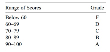
Let us suppose that in a biostatistics course, students are given a test that has 100 total possible points. Assume that the students who take this course have a normal distribution of scores with a mean of 75 and a standard deviation of 7. The instruc-tor uses the grading system presented in Table 6.1. Given this grading system and the assumed normal distribution, let us determine the percentage of students that will receive A, B, C, D, and F. This calculation will involve exercises with tables of the standard normal distribution.

First, let us repeat this table with the raw scores replaced by the Z scores. This process will make it easier for us to go directly to the standard normal tables. Recall that we arrive at Z by the linear transformation Z = (X – μ)/ σ. In this case μ = 75, σ = 7, and the X values we are interested in are the grade boundaries 60, 70, 80, and 90. Let us go through these calculations step by step for X = 90, X = 80, X = 70, and X = 60.

Step 1: Subtract μ from X: 90 – 75 = 15.

Step 2: Divide the result of step one by σ: 15/7 = 2.143 (The resulting Z score = 2.143)

Now take X = 80.

Step 1: Subtract μ from X: 80 – 75 = 5.

Step 2: Divide the result of step one by σ: 5/7 = 0.714 (Z = 0.714)

TABLE 6.1. Distribution of Grades in a Biostatistics Course

Now take X = 70.

Step 1: Subtract μ from X: 70–75 = –5.

Step 2: Divide the result of step one by σ: –5/7 = –0.714 (Z = –0.714)

Now take X = 60.

Step 1: Subtract μ from X: 60 – 75 = –15.

Step 2: Divide the result of step one by σ: –15/7 = –2.143 (Z = –2.143)

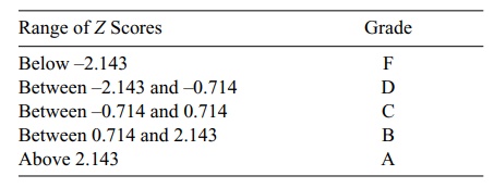
The distribution of percentiles and corresponding grades are shown in Table 6.2.

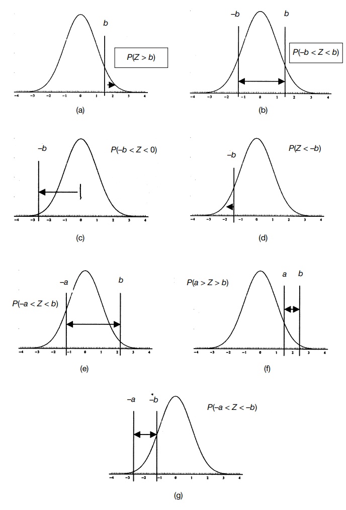
To determine the probability of an F we need to compute P(Z < –2.143) and find its value in a table of Z scores. The tables in our book (see Appendix D) give us P(0 < Z < b), where b is a positive number. Other probabilities are obtained using prop-erties of the standard normal distribution. These properties are given in Table 6.3. The areas associated with these properties are given in Figure 6.2.

Using the properties shown in the equations in Figure 6.2, Parts (a) through (g), we can calculate any desired probability. We are seeking probabilities on the left-hand side of each equation. The terms farthest to the right in these equations are the probabilities that can be obtained directly from the Z Table. (Refer to Appendix E.)

For P(Z < –2.143) we use the property in Part (d) and see that the result is 0.50-P(0 < Z < 2.143). The table of Z values is carried to only two decimal places. For greater accuracy we could interpolate between 2.14 and 2.15 to get the answer. But for sim-plicity, let us round 2.143 to 2.14 and use the probability that we obtain for Z = 2.14.

TABLE 6.2. Distribution of Z Scores and Grades

TABLE 6.3. Properties of the Table of Standard Scores (Used for Finding Z Scores)

a. P(Z > b) = 0.50 – P(0 < Z < b)

b. P(–b < Z < b) = 2P(0 < Z < b)

c. P(–b < Z < b) = P(0 < Z < b)

d. P(Z < –b) = P(Z > b) = 0.50 – P(0 < Z < b)

e. P(–a < Z < b) = P(0 < Z < a) + P(0 < Z < b), where a > 0

f. P(a < Z < b) = P(0 < Z < b) – P(0 < Z < a), where 0 < a < b

g. P(–a < Z < –b) = P(b < Z < a) = P(0 < Z < a) – P(0 < Z < b), where –a < –b < 0 and hence a > b > 0

Figure 6.2. The properties of Z Scores illustrated. Parts (a) through (g) illustrate the properties shown in Table 6.3. Note that b is symmetric. A negative letter (–a or –b) indicates that the Z score falls to the left of the mean, which is 0.

The Z table shows us that P(0 < Z < 2.14) = 0.4838. So the probability of getting an F is just 0.5000 – 0.4838 = 0.0162.

The probability of a D is P(–2.14 < Z < –0.71) by rounding to two decimal places. For this probability we must use the property in Part (g). So we have P(–2.14 < Z < –0.71) = P(0 < Z < 2.14) – P(0 < Z < 0.71) = 0.4838 – 0.2611 = 0.2227.

The probability of a C is P(–0.71 < Z < 0.71). Here we use property in Part (b).

We have P(–0.71 < Z < 0.71) = 2P(0 < Z < 0.71) = 2(0.2611) = 0.5222.

The probability of a B is P(0.71 < Z < 2.14). We could calculate this probability directly by using the property in Part (f). However, looking closely at Part (g), we see that it is the same as P(–2.14 < Z < –0.71), a probability that we have already calculated for a D. So we save some work and notice that the probability of a B is 0.2227.

The probability of an A is P(Z > 2.14). We can obtain this value directly from the property in Part (a). Again, if we look carefully at the property in Part (d), we see that P(Z > 2.14) = P(Z < –2.14), which equals the right-hand side that we calcu-lated previously for an F. So again, careful use of the properties can save us some work! The probability of an A is 0.0162.

We might feel that we are giving out too many Ds and Bs, possibly because the test is a little harder than the usual test for this class. If the instructor wants to adjust the test based on what the standard deviation should be (i.e., curve the test), the in-structor can make the following adjustments. The mean of 75 is where it should be, so only an adjustment is needed to take account of the spread of the score. If the ob-served mean were 70, an adjustment for this bias also could be made.

We will not go through the exercise of curving the tests, but let us see what would happen if we in fact did have a lower standard deviation of 5, for example, with an average of 75. In that case, what would we find for the distribution of grades?

We will repeat all the steps we went through before. The only difference will be in the final Z scores that we obtain, because we divide by 5 instead of 7.

Step 1: Subtract μ from X: 90 – 75 = 15

Step 2: Divide the result of step one by σ: 15/5 = 3.00. (The resulting Z score = 3.00.)

Now take X = 80.

Step 1: Subtract μ from X: 80 – 75 = 5

Step 2: Divide the result of step one by σ: 5/5 = 1.00 (Z = 1.00)

Now take X = 70.

Step 1: Subtract μ from X: 70 – 75 = –5

Step 2: Divide the result of step one by σ: –5/5 = –1.00 (Z = –1.00)

Now take X = 60.

Step 1: Subtract μ from X: 60 – 75 = –15

Step 2: Divide the result of step one by σ: –15/5 = –3.00 (Z = –3.00)

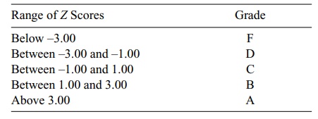
These results are summarized in Table 6.4. In this case we obtained whole integers that are easy to work with. Since we already know how to interpret 1s and 3s in terms of normal probabilities, we do not even need the tables but we will use them anyway.

We will use shorthand notation: P(F) = probability of receiving an F = P(Z < –3). Recall that by symmetry, P(F) = P(A) and P(D) = P(B). First compute P(A): P(A) = P(Z > 3) = 0.50-P(0 < Z < 3) = 0.50-0.4987 = 0.0013 = P(F).

Only about 1 in 1000 students will receive an F. Although the low number of Fs will please the students, an A will be nearly impossible! By symmetry, P(B) = P(1 < Z < 3) = P(0 < Z < 3) – P(0 < Z < 1) = 0.4987 – 0.3413 = 0.1574 = P(D). As a result, approximately 16% of the class will receive a B and 16% a D. These proportions of Bs and Ds represent fairly reasonable outcomes. Now P(C) = P(–1 < Z < 1) = 2 P(0 < Z < 1) = 2 (0.3413) = 0.6826. As expected, more than two-thirds of the class will receive the average grade of C.

Until now, you have learned how to use the Z table (Appendix E) by applying the seven properties shown in Table 6.3 to find grade distributions. In these exam-ples, we always started with specific endpoints or intervals for Z and looked up the probabilities associated with them. In other situations, we may know the specified probability for the normal distribution and want to look up the corresponding Z val-ues for an endpoint or interval.

Consider that we want to find a symmetric interval for a C grade on a test but we do not have specific cutoffs in mind. Rather, we specify that the interval should be centered at the mean of 75, be symmetric, and contain 62% of the population. Then P(C) should have the form: P(–a < Z < a) = 2P(0 < Z < a). We want P(C) = 0.62, so P(0 < Z < a) = 0.31. We now look for a value a that satisfies P(0 < Z < a) = 0.31. Scanning the Z table, we see that a value of a = 0.88 gives P(0 < Z < a) = 0.3106. That is good enough. So a = 0.88.