Population Distributions and the Distribution of Sample Averages from the Population

Sampling Distributions for Means

POPULATION DISTRIBUTIONS AND THE DISTRIBUTION OF SAMPLE AVERAGES FROM THE POPULATION

What is the strategy of statistical inference? Statistical inference refers to reaching conclusions about population parameters based on sample data. Statisticians make inferences based on samples from finite populations (even large ones such as the U.S. population) or conceptually infinite populations (a probability model of a distribution for which our sample can be thought of as a set of independent observations drawn from this distribution). Other examples of finite populations include all of the patients seen in a hospital clinic, all patients known to a tumor registry who have been diagnosed with cancers, or all residents of a nursing home.

As an example of a rationale for sampling, we note that it would be prohibitively expensive for a research organization to conduct a health survey of the U.S. popula-tion by administering a health status questionnaire to everyone in the United States. On the other hand, a random sample of this population, say 2000 Americans, may be feasible. From the sample, we would estimate health parameters for the popula-tion based on responses from the random sample. These estimates are random be-cause they depend on the particular sample that was chosen.

Suppose that we calculate a sample mean () as an estimate of the population mean (μ). It is possible to select many samples of size n from a population. The val-ue of this sample estimate of the parameter would differ from one random sample to the next. By determining the distribution of these estimates, a statistician is then able to draw an inference (e.g., confidence interval statement or conclusion of a hy pothesis test) based on the distribution of sample statistics. This distribution that is so important to us is called the sampling distribution for the estimate.

Similarly, we will observe for many different parameters of populations the sam-pling distribution of their estimates. First, we will start out with the simplest, name-ly, the sample estimate of a population mean.

Let us be clear on the difference between the sample distribution of an observa-tion and the sampling distribution of the mean of the observations. We will note that the parent populations for some data may have highly skewed distributions (either left or right), multimodal distributions, or a wide variety of other possible shapes. However, the central limit theorem, which we will discuss in this chapter, will show us that regardless of the shape of the distribution of the observations for the parent population, the sample average will have a distribution that is approximately a nor-mal distribution. This important result partially explains the importance in statistics of the normal or Gaussian distribution that we studied in the previous chapter.

We will see examples of data with distributions very different from the normal distribution (both theoretical and actual) and will see that the distribution of the av-erage of several samples, even for sample sizes as small as 5 or 10, will become symmetric and approximately normal—an amazing result! This result can be proved by using tools from probability theory, but that involves advanced probabil-ity tools that are beyond the scope of the course. Instead, we hope to convince you of the result by observing what the exact sampling distribution is for small sample sizes. You will see how the distribution changes as the sample size increases.

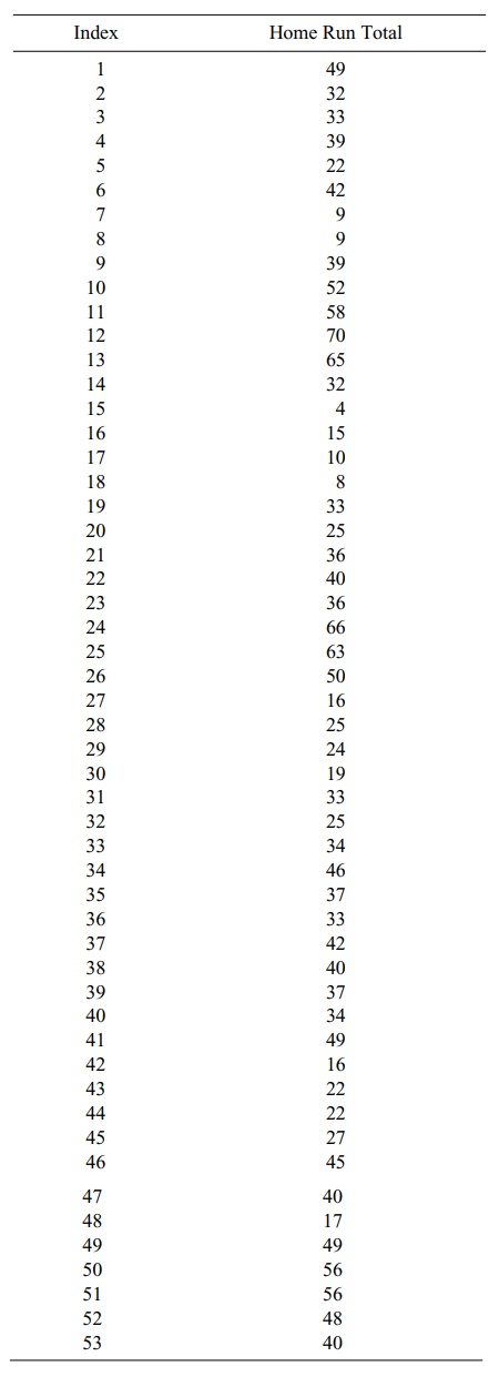
Recall from a previous exercise the seasonal home run totals of four current ma-jor league sluggers—Ken Griffey Jr, Mark McGwire, Sammy Sosa, and Barry Bonds. The home run totals for their careers, starting with their “rookie” season (i.e., first season with enough at bats to qualify as a rookie) is given as follows:

McGwire 49, 32, 33, 39, 22, 42, 9, 9, 39, 52, 58, 70, 65, 32

Sosa 4, 15, 10, 8, 33, 25, 36, 40, 36, 66, 63, 50

Bonds 16, 25, 24, 19, 33, 25, 34, 46, 37, 33, 42, 40, 37, 34, 49

Griffey 16, 22, 22, 27, 45, 40, 17, 49, 56, 56, 48, 40

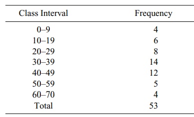
This gives us a total of 53 seasonal home run totals for top major league home run hitters. Let us consider this distribution (combining the totals for these four players) to be a population distribution for home run hitters. Now let us first look at a histogram of this distribution taking the intervals 0–9, 10–19, 20–29, 30–39, 40–49, 50–59, and 60–70 as the class intervals. Table 7.1 shows the histogram for these data.

The mean for this population is 35.26 and the population variance is 252.95. The population standard deviation is 15.90. These three parameters have been computed by rounding to two decimal places. Figure 7.1 is a bar graph of the histogram for this population.

We notice that although the distribution is not a normal distribution, it is not highly skewed either. Now let us look at the means for random samples of size 5.

TABLE 7.1. Histogram for Home run Hitters “Population” Distribution

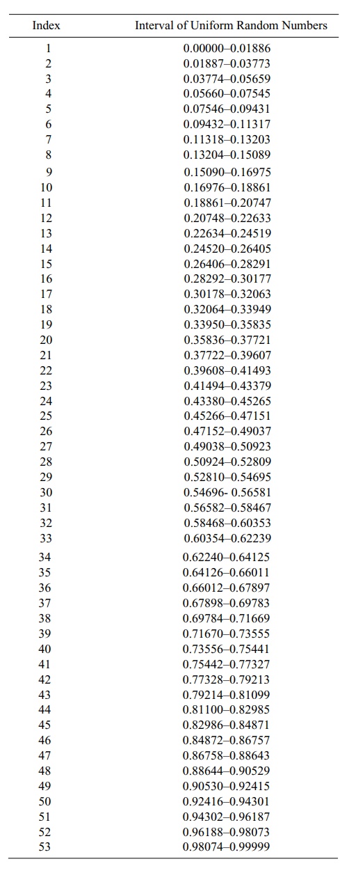
We shall use a random number table to generate 25 random samples each of size 5. For each sample we will compute the average and the sample estimate of standard deviation and variance. The indices for the 53 seasonal home run totals will be se-lected randomly from the table of uniform numbers. The indices correspond to the home run totals as shown in Table 7.2.

We sample across the table of random numbers until we have generated 25 sam-ples of size 5. For each sample, we are sampling without replacement. So if a par-ticular index is repeated, we will use the rejection sampling method that we learned in Chapter 2.

We refer to Table 2.1 for the random numbers. Starting in column row one and going across the columns and down we get the following numbers: 69158, 38683, 41374, 17028, and 09304. Interpreting these numbers as decimals 0.69158, 0.38683, 0.41374, 0.17028, and 0.09304 we then must determine the indices and decide whether we must reject any numbers because of repeats. To determine the indices, we divide the interval [0, 1] into 53 equal parts so that the indices correspond to random numbers in intervals as shown in Table 7.3.

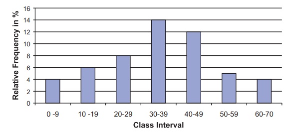
Figure 7.1. Relative frequency histogram for home run sluggers population distribution.

TABLE 7.2. Home Runs: Correspondence to Indices

Scanning Table 7.3 we find the following correspondences: 0.69158 → 37, 0.38683 → 21, 0.41374 → 22, 0.17028 → 10, and 0.09304 → 5. Since none of the indices repeated, we do not have to reject any random numbers and the first sample is obtained by matching the indices to home runs in Table 7.2.

We see that the correspondence is 37 → 42, 21 → 36, 22 → 40, 10 → 52, and 5 → 22. So the random sample is 42, 36, 40, 52, and 22. The sample mean, sample variance, and sample standard deviation rounded to two decimal places for this sample are 38.40, 118.80, and 10.90, respectively.

Although these numbers will vary from sample to sample, they should be com-parable to the population parameters. However, thus far we have computed only one sample estimate of the mean, namely, 38.40. We will focus attention on the dis-tribution of the 25 sample means that we generate and the standard deviation and variance for that distribution.

Picking up where we left off in Table 2.1, we obtain for the next sequence of 5 random numbers 10834, 10332, 07534, 79067, and 27126. These correspond to the indices 6, 6, 4, 42, and 15 respectively. Because 10332 led to a repeat of the index 6, we have to reject it and we complete the sample by adding the next number 00858 which corresponds to the index 1.

The second sample now consists of the indices 6, 4, 42, 15, and 1, and these in-dices correspond to the following homerun totals: 42, 39, 16, 4, and 49. The mean, standard deviation, and variance for this sample are 30.0, 19.09, and 364.50, respectively.

TABLE 7.3. Random Number Correspondence to Indices

We leave it to the reader to go through the rest of the steps to verify the remain-ing 23 samples. We will merely list the 25 samples along with their mean values:

1. 42 36 40 52 22 : 38.40

2. 423916449 : 30.00

3. 33 52 40 63 17 : 41.00

4. 837494028 : 31.80

5. 33 39 56 27 24 : 35.80

6. 45 48 49 10 66 : 43.60

7. 15 22 32 22 34 : 25.00

8. 37 46 56 16 33 : 37.60

9. 36940394 : 25.60

10. 42 39 34 17 33 : 33.00

11. 33 34 49 15 40 : 34.20

12. 34 52 56 42 24 : 41.60

13. 22 22 33 34 48 : 31.80

14. 15 39 22 16 50 : 28.40

15. 33 40 52 42 40 : 41.40

16. 40 42 45 49 16 : 38.40

17. 65 40 42 50 33 : 46.00

18. 253733498 : 30.40

19. 32 52 65 39 70 : 51.60

20. 49 50 39 40 25 : 40.60

21. 52 48 42 40 49 : 46.20

22. 42 40 66 33 25 : 41.20

23. 40 42 10 16 50 : 31.60

24. 946191734 : 25.00

25. 925583346 : 34.20

The average of the 25 estimates of the mean is 36.18, its sample standard deviation is 7.06, and the sample variance is 49.90.

Figure 7.2 shows the histogram for the sample means. We should compare it to the histogram for the original observations. The new histogram that we have drawn appears to be centered at approximately the same point but has a much smaller stan-dard deviation and is more symmetric, just like the histogram for a normal distribu-tion might look.

We note that the range of the averages is from 25 to 51.60, whereas the range of the original observations went from 4 to 70. The observations have a mean of 35.26, a standard deviation of 15.90, and a variance of 252.94, whereas the averages have a mean of 36.18, a standard deviation of 7.06, and a variance of 49.90.

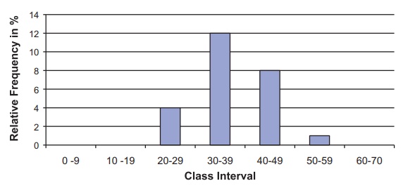
Figure 7.2. Relative frequency histogram for home run sluggers sample distribution for the mean of 25 samples.

We note that the means are close, differing only by 0.92 in absolute magnitude. The standard deviation is reduced by a factor of 15.90/7.06 ≈ 2.25 and the variance is reduced by a factor of 252.94/49.90 ≈ 5.07. This agrees very well with the theo-ry you will learn in the next two sections. Based on that theory, the average has the same mean as the original samples (i.e., it is an unbiased estimate of the population mean), the standard deviation for the mean of 5 samples is the population standard deviation divided by √5 ≈ 2.24, and the variance therefore by the population vari-ance divided by 5.

We compare these values based on comparing the population parameters to the observed samples with the theoretical values 0.92 to 0.00, 2.25 to 2.24, and 5.07 to 5.00. The reason that the results differ slightly from the theory is because we only took 25 random samples and therefore only got 25 averages for the distribu-tion. Had we done 100 or 1000 random samples, the observed results would have been closer to the theoretical results for the distribution of an average of 5 samples.

The histogram in Figure 7.2 does not look as symmetric as a normal distribution because we have a few empty class intervals and the filled ones are too wide. For the original data, we set up 7 class intervals for 53 observations that ranged from 4 to 70. For the means, we only have 25 values but their range is narrower—from 25 to 51.6. So we may as well take 7 class intervals of width 4 going from 24 to 52 as follows (see Figure 7.3):

Greater than or equal to 24 and less than or equal to 28

Greater than 28 and less than or equal to 32

Greater than 32 and less than or equal to 36

Greater than 36 and less than or equal to 40

Greater than 40 and less than or equal to 44

Greater than 44 and less than or equal to 48

Greater than 48 and less than or equal to 52.

Figure 7.3. Relative frequency histogram for home run sluggers sample distribution for the mean of 25 samples (new class intervals).

This picture is not as close to a normal distribution as the theory suggests. First of all, because we are only averaging 5 samples, the normal approximation will not be as good as if we averaged 20 or 50. Also, the histogram is only based on 25 samples. A much larger number of random samples might be necessary for the histogram to closely approximate the sampling distribution of the mean of 5 sample seasonal home run totals.