Student’s t Distribution Obtained When Standard Deviation Is Unknown

STUDENT’S t DISTRIBUTION OBTAINED WHEN STANDARD DEVIATION IS UNKNOWN

The Guinness Brewery in Dublin employed an English chemist, William Sealy Gosset, in the early 1900s. Gosset’s research involved methods for growing hops in order to improve the taste of beer. His experiments, which generally involved small samples, used statistics to compare hops developed by different procedures.

In his experiments, Gosset used Z statistics similar to the ones we have seen thus far (as in Formula 7.2). However, he found that the distribution of the Z statistic tended to have more extreme negative and positive values than one would expect to see from a standard normal distribution. This excess variation in the sampling dis-tribution was due to the presence of σ instead of σ in the denominator. The variabil-ity of σ, which depended on the sample size n, needed to be accounted for in small samples.

Eventually, Gosset was able to fit a Pearson distribution to observed values of his standardized statistic. The Pearson distributions were a large family of distribu-tions that could have symmetric or asymmetric shapes and have short or long tails. They were developed by Karl Pearson and were known to Gosset and other re-searchers. Instead of Z, we now use the notation t for the statistic that Gosset devel-oped. It turned out that Gosset had derived empirically the exact distribution for t when the sample observations have exactly a normal distribution. His t distribution provides the appropriate correction to Z in small samples where the normal distrib-ution does not provide an accurate enough approximation to the distribution of the sample mean because the effect of σ on the statistic matters.

Ultimately, tables similar to those used for the standard normal distribution were created for the t distribution. Unfortunately, unlike the standard normal, the distrib-ution of t changes as n changes (either increases or decreases).

Figure 7.5 shows how the shape of the t distribution changes as n increases. Three distributions are plotted on the graph, the t with 2 degrees of freedom, the t with 20 degrees of freedom, and the standard normal distribution. The term “de-grees of freedom” for a t distribution is a parameter denoted by “df ” that is equal to n – 1 where n is the sample size.

We can see from Figure 7.5 that the t is symmetric about zero but is more spread out than the standard normal distribution. Tables for the t distribution as a function of the percentile point of interest and the degrees of freedom are given in Appendix F. Formula 7.3 presents the t statistic.

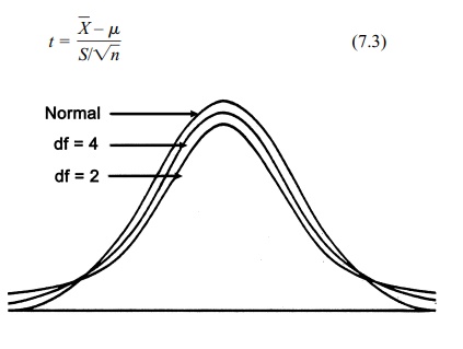
Figure 7.5. Comparison of normal distribution with t distributions of degrees of freedom (df ) 4 and 2. (Source: Adapted from Kuzma, J. W. Basic Statistics for the Health Sciences. Mountain View, Califor-nia: Mayfield Publishing Company, 1984, Figure 7.4, p. 84.)

For n ≤ 30, use the table of the t distribution with n – 1 degrees of freedom. When n > 30, there is very little difference between the standard normal distribution and the t distribution.

Let us illustrate the difference between Z and t with a medical example. We con-sider the blood glucose data from the Honolulu Heart Study (Kuzma, 1998, p. 93, Figure 7.1). The population distribution in this example, a finite population of N = 7683 patients, was highly skewed. The population mean and standard deviation were μ = 161.52 and σ = 58.15, respectively. Suppose we select a random sample of 25 patients from this population; what proportion of the sample would fall below 164.5?

First, let us use Z with μ and σ as given above (assumed to be known). Then Z = (164.5 – 161.52)/(58.15/√25) = 2.98/11.63 = 0.2562. Looking in Appendix E at the table for the standard normal distribution, we will use 0.26, since the table car-ries only two decimal places: P(Z > 0.26) = 0.5 – P(0 ≤ Z ≤ 0.26) = 0.5 – 0.1026 = 0.3974.

Suppose that (1) the mean μ is known to be 161.52, (2) the standard deviation σ is unknown, and (3) we use our sample of 25 to estimate σ. Although the sample estimate is not likely to equal the population value of 58.15, let us assume (for the sake of argument) that it does. When S = 58.15, t = 0.2562.

Now we must refer to Appendix E to determine the probability for a t with 24 degrees of freedom—P(t > 0.2562). As the table provides P(t ≤ a), in order to find P(t > a) we use the relationship that P(t > a) = 1 – P(t ≤ a); in our case, a = 0.2562. The table tells us that P(t ≤ 0.2562) = 0.60. So P(t > 0.2562) = 0.40. Note that there is not much difference between 0.40 for the t and the value 0.3974 that we obtained using the standard normal distribution. The reason for the similar results obtained for the t and Z distributions is that the degrees of freedom (df = 24) are close to 30.

Let us assume that n = 9 and repeat the foregoing calculations, this time for the probability of observing an average blood glucose level below 178.75. First, for Z we have Z = (178.75–161.52)/(58.15/√9) = 17.23/(58.15/3) = 17.23/19.383 = 0.889. Rounding 0.889 to two decimal places, P(Z < 0.89) = 0.50 + P(0 < Z < 0.89) = 0.50 + 0.3133 = 0.8133.

If we assume correctly that the standard deviation is estimated from the sample, we should apply the t distribution with 8 degrees of freedom. The calculated t statis-tic is again 0.889. Referencing Appendix F, we see for a t distribution with 8 de-grees of freedom P(t < 0.889) = 0.80. The difference between the probabilities ob-tained by the Z test and t test (0.8133 – 0.8000) equals 0.0133, or 1.33%. We see that because the t (df = 8) has more area in the upper tail than does the Z distribu-tion, the proportion of the distribution below 0.889 will be smaller than the propor-tion we obtained for a standard normal distribution.