The Central Limit Theorem

THE CENTRAL LIMIT THEOREM

Section 7.1 illustrated that as we average sample values (regardless of the shape of the distribution for the observations for the parent population), the sample average has a distribution that becomes more and more like the shape of a normal distribution (i.e., symmetric and unimodal) as the sample size increases. Figure 7.4, taken from Kuzma (1998), shows how the distribution of the sample mean changes as the sample size n increases from 1 to 2 to 5 and finally to 30 for a uni-form distribution, a bimodal distribution, a skewed distribution, and a symmetric distribution.

In all cases, by the time n = 30, the distribution in very symmetric and the variance continually decreases as we noticed for the home run data in the previous section. So, the figure gives you an idea of how the convergence depends on both the sample size n and the shape of the population distribution function.

What we see from the figure is remarkable. Regardless of the shape of the popu-lation distribution, the sample averages will have a nearly symmetric distribution approximating the normal distribution in shape as the sample size gets large! This is a surprising result from probability that is called the central limit theorem. Let us now state the results of the central limit theorem formally.

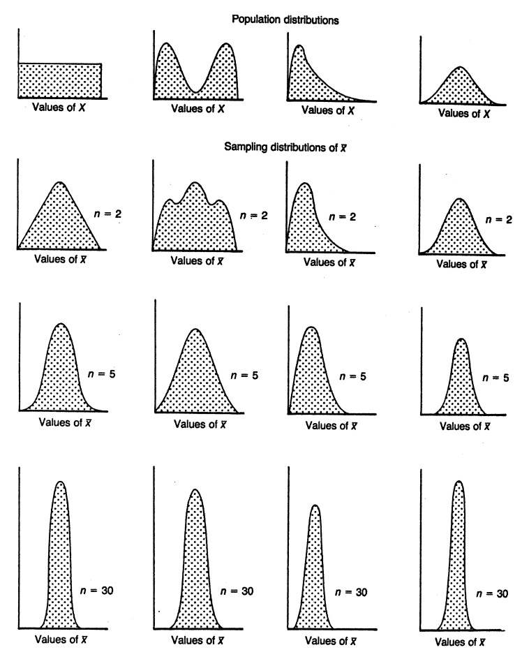
Figure 7.4. The effect of shape of population distribution and sample size on the distribution of means of random samples. (Source: Kuzma, J. W. Basic Statistics for the Health Sciences. Mountain View, California: Mayfield Publishing Company, 1984, Figure 7.3, p. 82.)

Suppose we have taken a random sample of size n from a population (generally, n needs to be at least 25 for the approximation to be accurate, but sometimes larger samples sizes are needed and occasionally, for symmetric populations, you can do fine with only 5 to 10 samples). We assume the population has a mean μ and a standard deviation σ. We then can assert the following:

1. The distribution of sample means  is approximately a normal distribution regardless of the population distribution. If the population distribution is nor-mal, then the distribution for  is exactly normal.

2. The mean for the distribution of sample means is equal to the mean of the population distribution (i.e., μ = μ where μ denotes the mean of the distri-bution of the sample means). This statement signifies that the sample mean is an unbiased estimate of the population mean.

3. The standard deviation of the distribution of sample means is equal to the standard deviation of the population divided by the square root of the sample size [i.e., σ = (σ/n), where σ is the standard deviation of the distribution of sample means based on n observations]. We call σ the standard error of the mean.

Property 1 is actually the central limit theorem. Properties 2 and 3 hold for any sam-ple size n when the population has a finite mean and variance.