Properties of Normal Distributions
| Home | | Advanced Mathematics |Chapter: Biostatistics for the Health Sciences: The Normal Distribution
The normal distribution has three main characteristics. First, its probability density is bell-shaped, with a single mode at the center.
PROPERTIES OF NORMAL DISTRIBUTIONS
The normal distribution has three main
characteristics. First, its probability density is bell-shaped, with a single
mode at the center. As the tails of the normal distribu-tion extend to ±∞`, the distribution decreases in height and remains
positive. It is symmetric in shape about μ, which is both its mean and mode. As detailed as this description may
sound, it does not completely characterize the normal distribution. There are
other probability distributions that are symmetric and bell-shaped as well. The
normal density function is distinguished by the rate at which it drops to zero.
Another parameter, σ, along with the mean, completes the characterization of the normal
distribution.
The relationship between σ and the area under the normal
curve provides the second main characteristic of the normal distribution. The
parameter σ is the
standard deviation of the distribution. Its square is the variance of the
distribution.
For a normal distribution, 68.26% of the probability
distribution falls in the interval from μ – σ to μ + σ. The wider interval from μ – 2σ to μ + 2 σ contains 95.45% of the
distribution. Finally, the interval from μ – 3σ to μ + 3σ contains 99.73% of the distribution, nearly 100% of the distribution.
The fact that nearly all observations from a normal distribution fall within ±3σ of the mean explains why the
three-sigma limits are used so often in practice.
Third, a complete mathematical
description of the normal distribution can be found in the equation for its
density. The probability density function f(x) for a nor-mal distribution is given
by

One awkward fact about the normal distribution is
that its cumulative distribution does not have a closed form. That means that
we cannot write down an explicit formula for it. So to calculate probabilities,
the density must be integrated numerically. That is why for many years
statisticians and other practitioners of statistical methods relied heavily on
tables that were generated for the normal distribution.
One important feature was very helpful in making
those tables. Although to specify a particular normal distribution one has to
provide the two parameters, the mean and the variance, a simple equation
relates the general normal distribution to one particular normal distribution
called the standard normal distribution.
For the general normal
distribution, we will use the notation N(μ, σ2). This ex-pression denotes a normal distribution
with mean μ and
variance σ2. The standard normal distribution has mean 0 and
variance 1. So N(0, 1) denotes the
standard nor-mal distribution. Figure 6.1 presents a standard normal
distribution with standard deviation units shown on the x-axis.
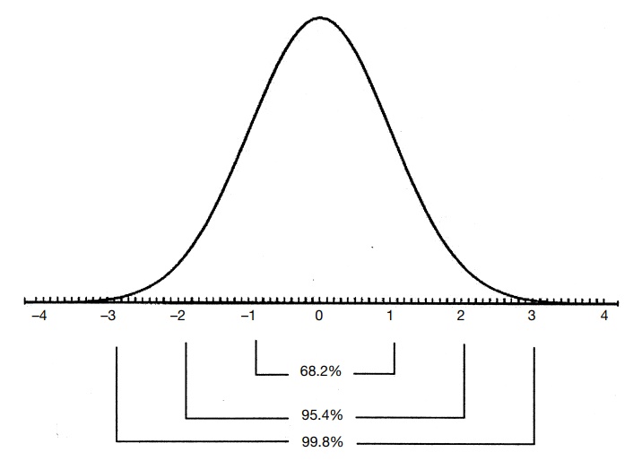
Figure 6.1. The standard normal distribution.
Suppose X
is N(μ, σ 2); if we let Z
= (X – μ)/σ, then Z is N(0,
1). The values for Z, an important
distribution for statistical inference, are available in a table. From the table, we can find the probability P for any values a < b, such that P(a ≤ Z ≤ b). But,
since Z = (X – μ)/σ, this is just P(a ≤ (X – μ)/σ ≤ b) = P(aσ ≤ (X – μ) ≤ bσ) = P(aσ + μ ≤ X ≤ bσ + μ). Thus, to make inferences about X,
all we need to do is to convert X to Z,
a process known as standardization.
So, probability statements about Z can be translated into probability
statements about X through this
relationship. Therefore, a single table for Z
suffices to tell us everything we need to know about X (assuming both μ and σ are specified).
Related Topics
