Exercises questions answers

EXERCISES

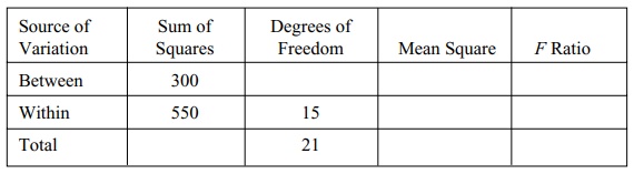
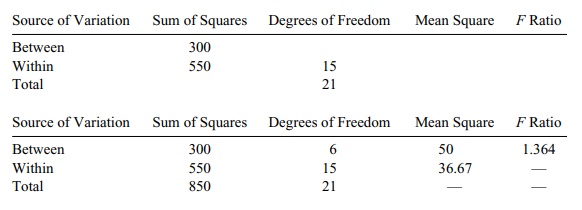
13.1 Complete the following ANOVA table:

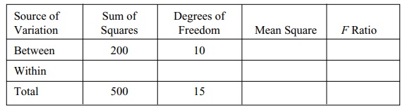
13.2 Complete the following ANOVA table:

13.3 Why does one use a Tukey’s HSD rather than a t test when comparing mean differences in ANOVA?

13.4 Samples were taken of individuals with each blood type to see if the average white blood cell count differed among types. Ten individuals in each group were sampled. The results are given in the table below:

Average White Blood Cell Count by Blood Type

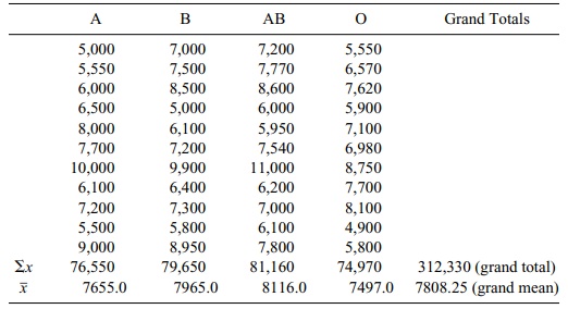
Source: Modification to Exercise 10.9, page 171, Kuzma and Bohnenblust (2001).

a. State the null hypothesis.

b. Construct an ANOVA table.

13.5 Using the data from the example in Exercise 13.4 and the ANOVA table from that exercise, determine the p-value for the test (use the F statistic and the appropriate degrees of freedom based on the within and between sum of squares). Is there a statistically significant difference in the white blood cell counts among the groups?

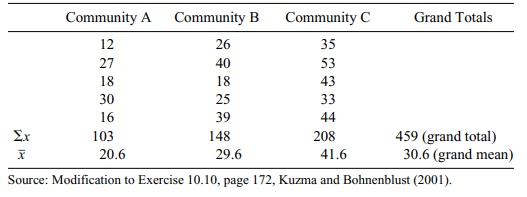
13.6 Five individuals were selected at random from three communities, and their ages were recorded in the table below. The investigator was interested in de-termining whether these communities differed in mean age.

Ages of Individuals (n = 5 in Each Group) in Three Communities

a. State the null hypothesis.

b. Construct an ANOVA table.

13.7 Using the data from the example in Exercise 13.6 and the ANOVA table from that exercise, determine the p-value for the test (use the F statistic and the appropriate degrees of freedom based on the within and between sum of squares). Is there a statistically significant difference in the ages among the groups?

13.8 Researchers studied the association between birth mothers’ smoking habits and the birth weights of their babies. Group 1 consisted of nonsmokers. Group 2 comprised smokers who smoked less than one pack of cigarettes per day. Group 3 smoked more than one but fewer than two packs per day. Group 4 smoked more than two packs per day.

Birth Weights of Infants (n = 11 in Each Group) by Mother’s Smoking Status

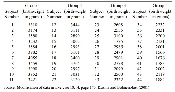
Use the above table to construct an ANOVA table for the test of no mean differences in birth weight among the groups. What is the p-value for this test? What do you conclude about the effect of smoking on birth weight?

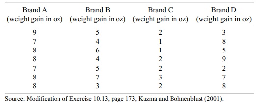
13.9 Four brands of cereal are compared to see if they produce significant weight gain in rats. Four groups of seven rats each were given a diet of the respective cereal brand. At the end of the experimental period, the rats were weighed and the weight was compared to the weight just prior to the start of the cereal diet. Determine whether each brand has a statistically significant effect on the amount of weight gain. The data are provided in the table below.

Rat Weight by Brand of Cereal

13.10 A botanist wants to determine the effect of microscopic worms on seedling growth. He prepares 16 identical planting pots and then introduces four sets of worm populations into them. There are four groups of pots with four pots in each group. The worm population group sizes are 0 (intro-duced into the first group of four pots), 500 (introduced into the second group of four pots), 1000 (introduced into the third group of four pots), and 4000 (introduced into the fourth group of four pots). Two weeks after planting, he measures the seedling growth in centimeters. The results are given in the table below.

Seedling Growth in Centimeters by Worm Population Group

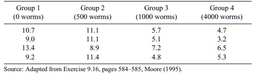
a. State the null hypothesis and determine the ANOVA table.

b. What is the result of the F test?

c. Apply Tukey’s HSD test to see which means differ if the ANOVA was significant at the 5% level.

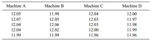
13.11 Analysis of variance may be used in an industrial setting. For example, man-agers of a soda-bottling company suspected that four filling machines were not filling the soda cans in a uniform way. An experiment on four machines doing five runs each gave the data in the following table.

Liquid Weight of Machine-Filled Cans in Ounces

Based on the analysis of variance, is there a difference in the average num-ber of ounces filled by the four machines? Apply Tukey’s HSD test to compare the mean differences if the overall ANOVA test is significant at the 5% level.

13.12 The following table shows the home run production of five of baseball’s greatest sluggers over a period of 10 years. Each has hit at least 56 home runs in a season and all but Griffey have had seasons with 60 or more. Sosa, Bonds, and Griffey are still active, McGwire has retired, and Ruth is de-ceased, so this time period constitutes the final 10 years of McGwire’s and Ruth’s respective careers.

Home Run Production for Five Great Sluggers

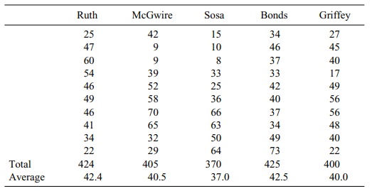
a. Construct an ANOVA table to test whether or not there are statistically significant differences in the home run production of these sluggers over the ten-year period.

b. If the F test indicates significant differences at the 0.05 significance level, apply Tukey’s HSD to see if there is a slugger who stands out with the lowest average. Is there a slugger with an average significantly higher than the rest? Is Bonds at 42.5 significantly higher than Sosa at 37.0?

Answers:

13.1 Complete the following ANOVA table:

13.3 Since we are looking at more than one pair of mean differences, there are multiple hypothesis tests, each having its own type I error. We want to control si-multaneously the type I errors that we could make. Tukey’s method guarantees that the probability of making a type I error on any of the tests is controlled to be less than α. A simple α-level t test on two or more mean differences would not provide such a control.

13.11 We construct an ANOVA table based on the data in the table below:

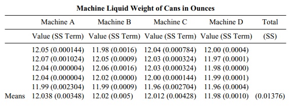
From above, the within-group sum of squares is 0.01376. The grand mean is 12.0125. So the between-group sum of squares is 5{(12.038 – 12.0125)² + (12.02 – 12.0125)² + (12.012 – 12.0125)² + (11.98 – 12.0125)²} = 5(0.00065025 + 0.00005625 + 0.00000025 + 0.00105625) = 5(0.001763) = 0.008815.

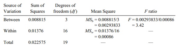
The result is significant at the 5% level since the critical f with 3 and 16 degrees of freedom is 3.24. So Tukey’s test is appropriate. Recall that HSD = q(α, k, N – k)  √(MS_w/n) where n is the number of observations per group, k is the number of groups, N = kn is the total sample size, and q(α, k, N – k) is gotten from Tukey’s table for the studentized range. In this case k = 4, n = 5, N = 20, and MS_W = 0.00086. So HSD = q(α, 4, 16) 0.01311. We take α = 0.05 and from the table get q = 4.05. So HSD = 0.0531. So we can reject the hypothesis that the two means are equal if their differences are 0.0531 or more. The mean differences are 0.018 for A minus B, 0.026 for A minus C, 0.058 for A minus D, 0.008 for B minus C, 0.040 for B minus D and 0.032 for C minus D. Note that only A minus D gives a value greater than HSD. So we conclude that D is less than A but cannot be confident about a differ-ence between any other pairs.