Wilcoxon Signed-Rank Test

WILCOXON SIGNED-RANK TEST

Remember that a paired t test involved taking the difference between two paired observations, i.e., d_i = X_it1 – X_it2. The Wilcoxon signed-rank test is a nonparametric rank test that is analogous to the paired t test but is applicable when the differences (d_i) between the two groups are not approximately normally distributed. The procedure of the Wilcoxon signed-rank test involves first computing the paired differ-ences, as with the t test. The absolute values of the differences are then computed and the data ranked based on these absolute differences. After the ranks are deter-mined, the observations are split into two distinct groups that separate the ones that have negative differences from the ones that have positive differences. The rank sums are then computed for the positive differences, with the test statistic denoted as T⁺. This test statistic is then compared to the tables for the signed-rank test; the tables are based on the distribution of this statistic when the central tendencies of the two populations are the same. Alternatively, we could have computed the sum of the negative ranks and denoted it by T^–.

If the two populations are the same, the paired differences will be symmetric about zero and therefore will have about the same number of positive and negative differences, and the magnitude of these differences will not depend on the sign (i.e., whether or not they are in the positive difference group). Assume that we find the differences between paired observations by subtracting the values for the second observation from the values for the first observation (as shown in Table 14.4). If the proportion of positive differences is high, it suggests that population one has a high-er median than population two. A low proportion of positive differences indicates that population one has a lower median than population two. In the event that a par-ticular paired difference is identical (i.e., 0), that observation is omitted from the calculation, and we proceed as if the number of pairs is one less than the original number.

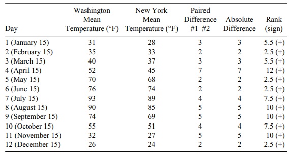
Recall from Chapter 9 the two cities data that we used to illustrate the paired t test. We will use these data to demonstrate how the signed-rank test works. (See Table 14.4.)

The fact that all the ranks are positive is a strong indicator that Washington was warmer than New York. This finding replicates the very highly significant differ-ence that was found using the paired t test.

The absolute value of the difference determines the ranks. The smallest absolute value gets rank 1, the next rank 2, and so on until we reach the largest with rank 12. However, in the example in Table 14.4 there is a tie for the lowest, with four cases having the value 2. When ties occur, all tied observations get the average of the tied ranks. So the average of ranks 1, 2, 3, and 4 is 10/4 = 2.5. Similarly the observed ab-solute difference of 3 is tied in two cases and hence the average of the ranks 5 and 6 gives a rank of 5.5 to each of those tied observations.

The sum of the positive ranks is 78, and the sum of the negative ranks is 0. Since n is small (12), we refer to the tables for the signed-rank test statistic. Recall that the sum of the positive ranks is denoted by T+. 

TABLE 14.4. Daily Temperatures, Washington versus New York

Referring to Appendix C, we find that for n = 12 and p = 0.005, the critical value is 8. This outcome means that the probability of observing a value less than 8 is 0.005. Similarly, from the tables the probability of observing a value greater than 70 is 0.005. This is based on symmetry since the prob-ability of the positive ranks being less than 8 under the null hypothesis is the same as the probability of being greater than 78 – 8 = 70. Since we observed a signed-rank score of 78, we know that the one-sided p-value is less than 0.005. So we conclude that there is a difference between the two populations in the mean temperature.

A normal approximation can be used for large n. Conover (1999) recommends that n be at least 50.

Let

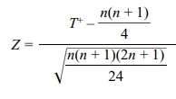
Then Z has approximately a standard normal distribution. So the standard normal tables (Appendix E) may be used after calculating Z in order to obtain an approxi-mate p-value for large n.

Another normal approximation that is simpler than the foregoing approximation is based on the statistic T = T⁺ – T^–. The statistic T has a mean of zero under the null hypothesis. So there is no expected value to subtract. For T (in the case when there are no ties) we define the standard normal approximation as

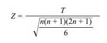
In the event of ties, we use Z = T/ √ΣR_i², where R_i is the absolute rank of the ith observation (both positive and negative ranks are included in this sum).

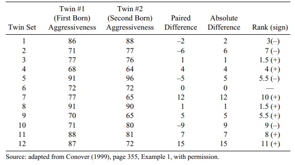
The temperature data (refer to Table 14.4) are highly unusual because of the ex-treme differences between the two cities; same-day pairing for each month of the year is used to remove the seasonal effect. As a second example of pairing, we will look at how twins score on a psychological test for aggressiveness (refer to Table 14.5). The data are from Conover (1999). The research question being addressed is whether first-born twins are more aggressive than second-born twins.

The value of n is 11 because we discard one pair of observations for which the difference is 0. Here we see that the sum of the ranks for a sample size of 11 is 66 (1 + 2 + 3 + . . . + 11). From the paired difference column, we see that the sum of the positive ranks is 41.5 and the sum of the negative ranks is 24.5. From the table for the signed-rank test with n = 11 (Appendix C), we see that the critical value at the one-sided 5% significance level is 55. Given that the sum of the positive ranks is 41.5, we cannot reject the null hypothesis because the p-value is greater than 0.05. Therefore, first-born twins do not tend to be more aggressive than second-born twins.

TABLE 14.5. Aggressiveness Scores for 12 Sets of Identical Twins

The normal approximations for the signed-rank test, recommended when n is 50 or more, are summarized in Equations 14.3 (no ties) and 14.4 (ties). A normal approximation to the Wilcoxon signed-rank test for comparing two dependent sam-ples (no ties) is

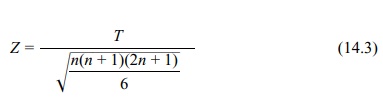
where T = T ⁺ – T ^– is the sum of the ranks, and n is the common sample size for both population 1 and population 2. A normal approximation to the wilcoxon signed-rank test for comparing two independent samples (ties) is

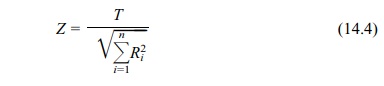
where T ⁺ – T ^– is the sum of the ranks, Σⁿ_i=1R²_i is the sum of the squares of the absolute ranks, and n is the common sample size for both population 1 and population 2.