F Distribution and Applications

F DISTRIBUTION AND APPLICATIONS

The F distribution will be used to evaluate the significance of the association between an independent variable and an outcome variable in an ANOVA. The F distribution is defined as the distribution of (Z/n₁)/(W/n₂), where Z has a chi-square distribution with n₁ degrees of freedom, W has a chi-square distribution with n₂ degrees of freedom, and Z and W are statistically independent. In the one-way analysis of variance, Z = Q₂/σ², W = Q₁/σ², n₁ = n_w, and n₂ = n_b – 1; so the ratio [Q₂/(n_b – 1)]/[Q₁/n_w] has the central F distribution with n_b – 1 numerator degrees of freedom and n_w denominator degrees of freedom under the null hypothesis. Note that the common variance σ² appears in both the numerator and denominator and hence cancels out of the ratio.

The probability density function for this F distribution has been derived and is described in statistical texts [see page 246 in Mood, Graybill, and Boes (1974)].

TABLE 13.1. General One-Way ANOVA Table

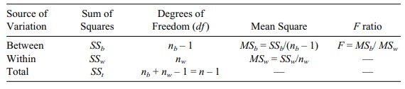
The F distribution depends on the two degrees of freedom parameters n₁ and n₂, called, respectively, the numerator and denominator degrees of freedom. We in-clude tables of the central F distribution based on degree of freedom parameters in Appendix A. A sample ANOVA is presented in Table 13.1.

Although we do not cover the two-way analysis of variance, Table 13.2 shows the typical two-way ANOVA table that should help you see how the ANOVA table generalizes to N-way ANOVAs. Note that as more factors appear, we have more than one F test. This appearance of multiple F tests is analogous to the several F and/or t tests in regression that are used to determine the significance of the regres-sion coefficients. ANOVA Table 13.2 is not the most general table. A treatment by block effect also can be considered in the model; in this case, the table would have another row for the interaction term.

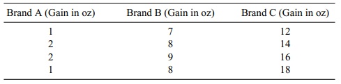
We will illustrate the one-way analysis of variance with a numerical example. Table 13.3 shows some hypothetical data for the weight gain of pigs fed with three different brands of cereal. A total of 12 pigs are randomly assigned (4 each) to the three cereal brands.

To generate the ANOVA table, we must calculate SS_b and SS_w. As a first step in obtaining SS_w, we calculate the means for each brand. _A = (1 + 2 + 2 + 1)/4 = 1.5. _B = (7 + 8 + 9 + 8)/4 = 8. _C = (12 + 14 + 16 + 18)/4 = 15. The grand mean is X = (1.5 + 8 + 15)/3 = 8.167. Now SS_W = Q₁ = (1 – 1.5)² + (2 – 1.5)² + (2 – 1.5)² + (1–1.5)²+(7–8)²+(8–8)²+(9–8)²+(8–8)²+(12–15)²+(14–15)²+ (16–15)²+(18–15)²=0.25+0.25+0.25+0.25+1+0+1+0+9+1+1+9= 23. Note that SS_w represents the sum of squared deviations of the individual observa-tions from their group means.

Now let us compute SS_b. We can calculate this directly or calculate SS_t and get SS_b by the equation SS_b = SS_t – SS_w. Since SS_t is a little easier to compute, let us do it by the subtraction method first. 

TABLE 13.2. Typical Two-Way ANOVA Table

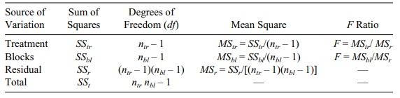
TABLE 13.3. Weight Gain for 12 Pigs Fed with Three Brands of Cereal

We need to get the overall or “grand” mean—the weighted average of the group means weighted by their respective sample sizes. In this case, since all three groups have 4 pigs each, the result is the same as taking the arithmetic average of the three group averages. So _g = (1.5 + 8 + 15)/3 = 8.1667. For SS_t, we do the same computations as for SS_w except that instead of subtracting the group means, we subtract the grand mean before taking the square. So for SS_t we have SS_t = Q = (1 – 8.1667)² + (2 – 8.1667)² + (2 – 8.1667)² + (1 – 8.1667)² + (7 - 8.1667)² + (8 – 8.1667)² + (9 – 8.1667)² + (8 – 8.1667)² + (12 – 8.1667)² + (14 – 8.1667)² + (16 – 8.1667)² + (18 – 8.1667)² = 51.3616 + 38.0282 + 38.0282 + 51.3616 + 2.7789 + 0.0278 + 0.6944 + 0.0278 + 14.6942 + 34.0274 + 61.3606 + 96.6938 = 391.0845.

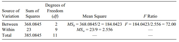
So by subtraction, SS_b = 391.0845–23.0 = 368.0845. Now we can fill in the ANOVA table. Table 13.4 is the ANOVA table of the form of Table 13.1 as applied to these data.

An F statistic of 72.00 is highly significant. Compare it to values in the F distri-bution table with 2 degrees of freedom in the numerator and 9 degrees of freedom in the denominator (Appendix A). The critical values are 4.26 at the 5% level and 8.02 at the 1% level. So we see that the p-value is considerably less than 0.01.

SS_b can be calculated directly. The formula is n_ob{(_A –)² + (_B – )² + (_C – )²} = 4{(1.5 – 8.167)² + (8 – 8.167)² + (15 – 8.167)²} = 4{44.444 + 0.0279 + 46.690} = 364.647. This formula applies to balanced designs where n_ob is the com-mon number of observations in each group. The difference between the results ob-tained from the two methods for calculating SS_b (364.667 versus 364.647) is due to rounding errors. Using SAS software and applying the GLM procedure to these data, we found that SS_b = 364.667. So most of the rounding error was in our calcu-lation of SS_t in the first approach.

TABLE 13.4. One-Way ANOVA Table for Pig Feeding Experiment