Design of Dosage Regimens

DESIGN OF DOSAGE REGIMENS

Dosage regimen is defined as the manner in which a drug is taken. For some drugs like analgesics, hypnotics, antiemetics, etc., a single dose may provide effective treatment. However, the duration of most illnesses is longer than the therapeutic effect produced by a single dose. In such cases, drugs are required to be taken on a repetitive basis over a period of time depending upon the nature of illness. Thus, for successful therapy, design of an optimal multiple dosage regimen is necessary. An optimal multiple dosage regimen is the one in which the drug is administered in suitable doses (by a suitable route), with sufficient frequency that ensures maintenance of plasma concentration within the therapeutic window (without excessive fluctuations and drug accumulation) for the entire duration of therapy. For some drugs like antibiotics, a minimum effective concentration should be maintained at all times and for drugs with narrow therapeutic indices like phenytoin, attempt should be made not to exceed toxic concentration.

Approaches to Design of Dosage Regimen

The various approaches employed in designing a dosage regimen are –

1. Empirical Dosage Regimen – is designed by the physician based on empirical clinical data, personal experience and clinical observations. This approach is, however, not very accurate.

2. Individualized Dosage Regimen – is the most accurate approach and is based on the pharmacokinetics of drug in the individual patient. The approach is suitable for hospitalised patients but is quite expensive.

3. Dosage Regimen on Population Averages – This is the most often used approach. The method is based on one of the two models –

(a) Fixed model – here, population average pharmacokinetic parameters are used directly to calculate the dosage regimen.

(b) Adaptive model – is based on both population average pharmacokinetic parameters of the drug as well as patient variables such as weight, age, sex, body surface area and known patient pathophysiology such as renal disease.

In designing a dosage regimen based on population averages —

1. It is assumed that all pharmacokinetic parameters of the drug remain constant during the course of therapy once a dosage regimen is established. The same becomes invalid if any change is observed.

2. The calculations are based on open one-compartment model which can also be applied to two compartment model if β is used instead of K_E, and V_d,ss instead of V_d while calculating the regimen.

Irrespective of the route of administration and complexity of pharmacokinetic equations, the two major parameters that can be adjusted in developing a dosage regimen are —

1. The dose size — the quantity of drug administered each time, and

2. The dosing frequency — the time interval between doses.

Both parameters govern the amount of drug in the body at any given time.

Dose Size

The magnitude of both therapeutic and toxic responses depends upon dose size. Dose size calculation also requires the knowledge of amount of drug absorbed after administration of each dose. Greater the dose size, greater the fluctuations between C_ss,max and C_ss,min during each dosing interval and greater the chances of toxicity (Fig. 12.1). For drugs administered chronically, dose size calculation is based on average steady state blood levels and is computed from equation 12.8.

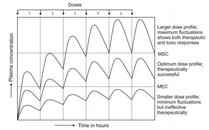
Fig. 12.1 Schematic representation of influence of dose size on plasma concentration-time profile after oral administration of a drug at fixed intervals of time.

Dosing Frequency

The dose interval (inverse of dosing frequency) is calculated on the basis of half-life of the drug. If the interval is increased and the dose is unchanged, C_max, C_min and C_av decrease but the ratio C_max/C_min increases. Opposite is observed when dosing interval is reduced or dosing frequency increased. It also results in greater drug accumulation in the body and toxicity (Fig. 12.2).

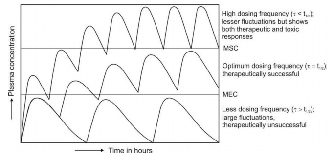
Fig. 12.2 Schematic representation of the influence of dosing frequency on plasma concentration-time profile obtained after oral administration of fixed doses of a drug.

A proper balance between both dose size and dosing frequency is often desired to attain steady-state concentration with minimum fluctuations and to ensure therapeutic efficacy and safety. The same cannot be obtained by giving larger doses less frequently. However, administering smaller doses more frequently results in smaller fluctuations.

Generally speaking, every subsequent dose should be administered at an interval equal to half-life of the drug. A rule of thumb is that –

^·            For drugs with wide therapeutic index such as penicillin, larger doses may be administered at relatively longer intervals (more than the half-life of drug) without any toxicity problem

^·            For drugs with narrow therapeutic index such as digoxin, small doses at frequent intervals (usually less than the half-life of the drug) is better to obtain a profile with least fluctuations which is similar to that observed with constant rate infusion or controlled-release system.

Drug Accumulation During Multiple Dosing

Consider the amount of drug in the body-time profile shown in Fig. 12.3. obtained after i.v. multiple dosing with dosing interval equal to one t_½.

After the administration of first dose X_o at τ = 0, the amount of drug in the body will be X = 1X_o. At the next dosing interval when X = ½X_o, the amount of drug remaining in the body, administration of the next i.v. dose raises the body content to X = X_o + ½X_o i.e. drug accumulation occurs in the body. Thus, accumulation occurs because drug from previous doses has not been removed completely. As the amount of drug in the body rises gradually due to accumulation, the rate of elimination also rises proportionally until a steady-state or plateau is reached when the rate of drug entry into the body equals the rate of exit. The maximum and minimum values of X i.e. X_ss,max and X_ss,min approach respective asymptotes at plateau. It is interesting to note that at plateau, X_ss,min = 1X_o and X_ss,max = 2X_o i.e. X_ss,min equals the amount of drug in the body after the first dose and X_ss,max equals twice the first dose. Also (X_ss,max – X_ss,min) = X_o and X_ss,max/X_ss,min = 2. All this applies only when τ  = t_½ and drug is administered intravenously. When τ < t_½, the degree of accumulation is greater and vice-versa.

Thus, the extent to which a drug accumulates in the body during multiple dosing is independent of dose size, and is a function of –

^·            Dosing interval, and

^·            Elimination half-life.

The extent to which a drug will accumulate with any dosing interval in a patient can be derived from information obtained with a single dose and is given by accumulation index R_ac as:

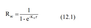
Fig.12.3 Accumulation of drug in the body during multiple dose regimen of i.v. bolus with dosing interval equal to one half-life of the drug. Approximately 5 half-lives are required for attainment of steady-state.

Time to Reach Steady-State During Multiple Dosing

The time required to reach steady-state depends primarily upon the half-life of the drug. Provided K_a >> K_E, the plateau is reached in approximately 5 half-lives. This is called as plateau principle. It also means that the rate at which the multiple dose steady-state is reached is determined only by K_E. The time taken to reach steady-state is independent of dose size, dosing interval and number of doses.

Maximum and Minimum Concentration During Multiple Dosing

If n is the number of doses administered, the C_max and C_min obtained on multiple dosing after the nth dose is given as:

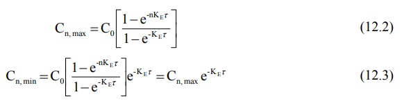
The maximum and minimum concentration of drug in plasma at steady-state are found by following equations:

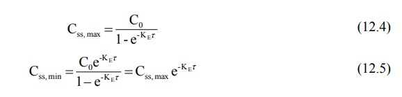
where C_o = concentration that would be attained from instantaneous absorption and distribution (obtained by extrapolation of elimination curve to time zero). Equations 12.2 to 12.5 can also be written in terms of amount of drug in the body. Fraction of dose absorbed, F, should be taken into account in such equations.

Fluctuation is defined as the ratio C_max/C_min. Greater the ratio, greater the fluctuation. Like accumulation, it depends upon dosing frequency and half-life of the drug. It also depends upon the rate of absorption. The greatest fluctuation is observed when the drug is given as i.v. bolus. Fluctuations are small when the drug is given extravascularly because of continuous absorption.

Average Concentration and Body Content on Multiple Dosing to Steady-State

The average drug concentration at steady-state C_ss,av is a function of –

·           The maintenance dose X_o,

·           The fraction of dose absorbed F,

·           The dosing interval τ and

·           Clearance Cl_T (or V_d and K_E or t_½) of the drug.

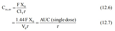
where the coefficient 1.44 is the reciprocal of 0.693 in equation 12.7. AUC is the area under the curve following a single maintenance dose. Equation 12.7 can be used to calculate maintenance dose of a drug to achieve a desired concentration. Since X = V_d C, the body content at steady-state is given as:

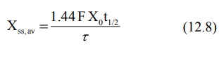
These average values are not arithmetic mean of C_ss,max and C_ss,min since the plasma drug concentration declines exponentially.

Loading and Maintenance Doses

A drug does not show therapeutic activity unless it reaches the desired steady-state. It takes about 5 half-lives to attain it and therefore the time taken will be too long if the drug has a long half-life. Plateau can be reached immediately by administering a dose that gives the desired steady-state instantaneously before the commencement of maintenance doses X_o.

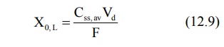
Such an initial or first dose intended to be therapeutic is called as priming dose or loading dose X_o,L. A simple equation for calculating loading dose is:

After e.v. administration, C_max is always smaller than that after i.v. administration and hence loading dose is proportionally smaller. For drugs having low therapeutic indices, the loading dose may be divided into smaller doses to be given at various intervals before the first maintenance dose. When V_d is not known, loading dose may be calculated by the following equation:

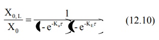
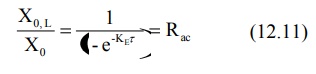
The above equation applies when K_a >> K_E and drug is distributed rapidly. When the drug is given i.v. or when absorption is extremely rapid, the absorption phase is neglected and the above equation reduces to accumulation index:

The ratio of loading dose to maintenance dose X_o,L/X_o is called as dose ratio. As a rule, when τ = t_½, dose ratio should be equal to 2.0 but must be smaller than 2.0 when τ  > t_½ and greater when τ < t_½. Fig. 12.4. shows that if loading dose is not optimum, either too low or too high, the steady-state is attained within approximately 5 half-lives in a manner similar to when no loading dose is given.

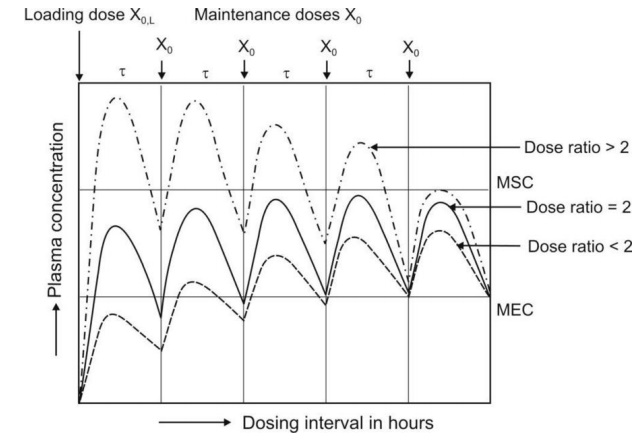
Fig. 12.4 Schematic representation of plasma concentration-time profiles that result when dose ratio is greater than 2.0, equal to 2.0 and smaller than 2.0.

The foregoing discussion and the equations expressed until now apply only to drugs that follow one-compartment kinetics with first-order disposition. Equations will be complex for multicompartment models.

Maintenance of Drug within the Therapeutic Range

The ease or difficulty in maintaining drug concentration within the therapeutic window depends upon —

1. The therapeutic index of the drug

2. The half-life of the drug

3. Convenience of dosing.

It is extremely difficult to maintain such a level for a drug with short half-life (less than 3 hours) and narrow therapeutic index e.g. heparin, since the dosing frequency has to be essentially less than t_½. However, drugs such as penicillin (t_½ = 0.9 hours) with high therapeutic index may be given less frequently (every 4 to 6 hours) but the maintenance dose has to be larger so that the plasma concentration persists above the minimum inhibitory level.

A drug with intermediate t_½ (3 to 8 hours) may be given at intervals τ ≤ t_½ if therapeutic index is low and those with high indices can be given at intervals between 1 to 3 half-lives. Drugs with half-lives greater than 8 hours are more convenient to dose. Such drugs are usually administered once every half-life. Steady-state in such cases can be attained rapidly by administering a loading dose. For drugs with very long half-lives (above 24 hours) e.g. amlodipine, once daily dose is very convenient.

Design of Dosage Regimen from Plasma Concentrations

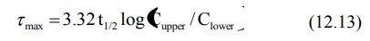
If the therapeutic range, apparent V_d and clearance or half-life of a drug is known, then dosage regimen can be designed to maintain drug concentration within the specified therapeutic range. The latter is defined by lower limit (C_lower) and an upper limit (C_upper). The maximum dosing interval, which ideally depends upon the therapeutic index (can be defined as a ratio of C_upper to C_lower) and elimination half-life of the drug, can be expressed by equation 12.12, a modification of equation 12.5.

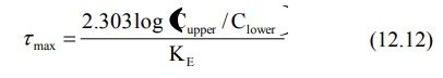
Since K_E = 0.693/t_½, the above equation can also be written as:

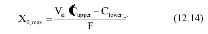
Understandably, the dosing interval selected is always smaller than τ_max. The maximum maintenance dose Xo,max that can be given every τ_max is expressed as:

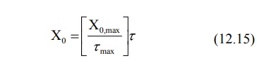
After a convenient dosing interval τ, smaller than τ_max has been selected, the maintenance dose is given as:

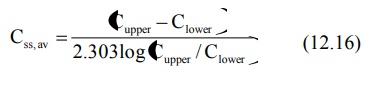
Administration of Xo every τ produces an average steady-state concentration defined by equation 12.7. The value of Css,av can also be calculated from the therapeutic range according to equation 12.16.