Exercises questions answers

EXERCISES

15.1 Give definitions of the following terms in your own words and indicate when it is appropriate to use each of them.

a.     Life tables

b.     The Kaplan–Meier curve

c.      The negative exponential survival distribution

d.     The Weibull distribution

e.      Cure rate models

f.       Log rank test

15.2 For a negative exponential survival function S(t), recall that S(t) = exp(λt), where λ is the rate parameter or hazard rate function. Consider the conditional probability that the survival time is T > t₂, given that we know T > t₁, where t₁ < t₂. Denote by S(t₂|t₁) the conditional probability of survival be-yond t₂, given that the patient survives beyond t₁, i.e., P[T > t₂|T > t₁]. Show that S(t₂|t₁) = exp[λ(t₂ – t₁)]. The term exp[λ(t₂ – t₁)] is called the lack of memory property of the negative exponential lifetime model because the survival at time t₁ has the same distribution as the survival at time 0; if τ = t₂ - t₁, the probability of surviving τ units of time is the same at 0 as it is at t₁, namely exp(λt). The probability of surviving depends only on τ and not on the time t₁ that we are conditioning on.

15.3 If the survival function S(t) = 1 – t/b for 0 ≤ t ≤ b for a fixed positive con-stant b, calculate the hazard function h(t) for 0 ≤ t ≤ b. Recall that F(t) = 1 - S(t) and f (t) is the derivative of F with respect to t. By definition, h(t) = f (t)/S(t). What is the lowest value for the hazard rate? Is there a highest val-ue for the hazard rate? (Hint: Choose M large. If there exists a c < b such that h(c) is greater than M and M is arbitrary, then there is no highest value for the hazard function.)

15.4 If the survival times in months for one group are {7.5, 12, 16, 33⁺, 55, 61} and {31, 60, 65, 76⁺, 80⁺, 92} for the second group, apply the chi-square test to see if the survival curves are significantly different from one another. Re-call that the notation of a plus as a superscript on the number indicates cen-soring at the denoted time, namely at 33 months for the case in group 1 and at 76 and 80 months for the cases in group 2. Test at the 0.01 significance level. Does the result seem obvious just from looking at the data?

15.5 Suppose the survival times (in months since transplant) for eight patients who received bone marrow transplants are 3.0, 4.5, 6.0, 11.0, 18.5, 20.0, 28.0, and 36.0. Assume no censoring.

a.     What is the median survival time?

b.     What is the mean survival time?

c.      Using 5 months as the interval, construct a life table for these data.

15.6 Using the data in Exercise 15.5,

a.     Calculate a Kaplan–Meier curve for the survival distribution.

b.     Fit a negative exponential survival model to the data.

c.      Compare the fitted exponential to the Kaplan–Meier curve at the eight event times.

d.     Based on the comparison in c, would you say the exponential is a good fit?

15.7 Again, we use the data from Exercise 15.5, but we assume that 6.0, 18.5, and 28 are censor times.

a.     Estimate the median survival time.

b.     Why would an estimate of the mean survival time based on averaging all the times be inappropriate?

c.      Using 5 months as an interval, construct a life table for the data.

15.8 Using the data in Exercise 15.7, construct a Kaplan–Meier estimate of the survival distribution.

15.9 Again using the data in Exercise 15.7, fit a negative exponential model. Compare it to the Kaplan–Meier curve at the event times 3, 4.5, 11.0, 20.0, and 36.0 months, and decide whether or not the negative exponential pro-vides a good fit.

15.10 Using a chi-square test, formally test the goodness of fit of the negative ex-ponential distribution obtained in Exercise 15.9. Test at the 0.05 level of sig-nificance.

15.11 Listed below in units of months are the survival and censor times (censoring denoted by a superscripted plus sign) for six males and six females.

Males: 1, 3, 4⁺, 9, 11, 17

Females: 1, 3⁺, 6, 9, 10, 11⁺

a.     Calculate a Kaplan–Meier curve for the males.

b.     Calculate a Kaplan–Meier curve for the females.

c.      Apply a chi-square test to determine if the two survival curves differ from one another.

15.12 For the data in Exercise 15.11:

a.     Compute the mean survival time for males using all the observations (in-cluding the censoring times).

b.     Repeat part a for the females.

c.      Compute the mean survival times for males and females, respectively, using only the uncensored times.

d.     Which estimate makes more sense if censoring can be considered to oc-cur at random?

Answers:

15.2 S(t₂|t₁) = P{T > t₂|T > t₁} = P{T > t₂ ∩ T > t₁}/P{T > t₁}. Since t₂ > t₁, the event T > t₂ is contained in the event T > t₁. Therefore P{T > t₂ ∩ T > t₁} = P{T > t₂}. So S(t₂|t₁) = P{T > t₂}/P{T > t₁} = exp(λt₂)/exp(λt₁) = exp(λt₂ – λt₁) = exp[λ(t₂ – t₁)].

15.4 We get the expected and observed numbers for the chi-square test from the following table:

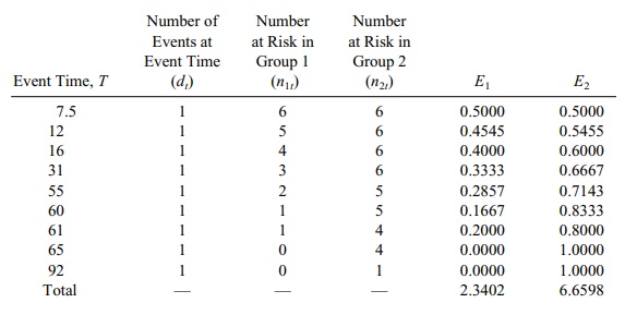
Now for the chi-square, we have the observed number of 5 events for group 1 and 5 events for group 2. So χ² = (5 – 2.3402)²/2.3402 + (5 – 6.6598)²/6.6598 = 3.437. This does not quite reach the 5% level of significance. The distributions do appear to differ by inspection, but the sample size is small (only 5 events in each group).

15.6 a. We generate the Kaplan–Meier curve using the following table:

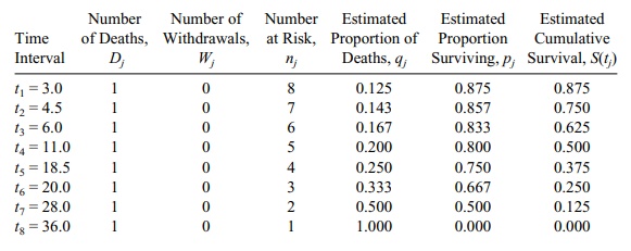
b and c. For the negative exponential, S(t) = exp(–λt) and we estimate time between failures 1/λ from the data as total time on test divided by the total number deaths = (3.0 + 4.5 + 6.0 + 11.0 + 18.5 + 20.0 + 28.0 + 36.0)/8 = 127/8 = 15.875. So the estimate for λ = 1/15.875 = 0.063.

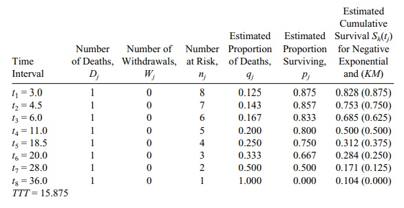
d. This exponential model seems to reasonably fit the data.

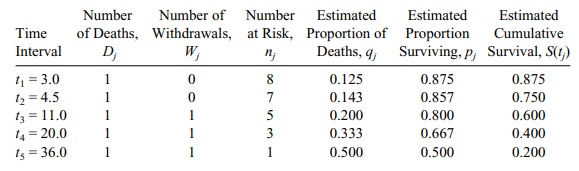
15.8 Here we change the events at times 6.0, 18.5, and 28.0 to censored times rather than event times. The corresponding Kaplan–Meier table looks as follows: