Survival Probabilities: Parametric Survival Curves

Parametric Survival Curves

If we give the survival function a specific functional form, we can estimate the survival curve based on just a few parameter estimates. We will illustrate this proce-dure with the negative exponential and Weibull distributions.

The negative exponential, a simple one-parameter family of probability distribu-tions, models well the lifetime distributions for some products, such as electric light bulbs; i.e., it is useful in describing their time to failure.

The Weibull distribution is a two-parameter family of distributions that has been used even more widely than the negative exponential to model time to failure for manufactured products. The Weibull distribution shares one major characteristic with the normal distribution model; i.e., it is a limiting distribution. Each distribu-tion is successful under certain circumstances.

Whereas the normal distribution is a limiting distribution for sums or averages of independent observations with the same distribution, the Weibull is a limiting dis-tribution for the smallest value in a sample of independent observations with the same distribution.

Recall that in Chapter 7 we saw that as the sample size (n) increases, the sam-pling distribution of means becomes more and more similar to a normal distribu-tion. Because the distribution continues to become close to the normal distribution as the sample size increases, we call the normal distribution a limiting distribution. Similarly, if we have a sample of size n, the probability distribution for the smallest value among the n observations approaches the Weibull distribution more closely as the sample size n increases. To obtain standard forms for the Weibull as we did with the normal distribution, we subtract a constant from the original statistic (e.g., minimum value in the sample) and then divide the result by another constant.

This procedure is analogous to Z = (X – μ)/(σ/√n) for the standard normal dis-tribution. The normal distribution works well when the variable of interest can be viewed as a sum. The Weibull works well when the variable of interest can be viewed as the smallest value.

For mortality, we can think of time to death as the time when an illness, exposure factor, or other occurrence causes a person to die. Mortality can be modeled in terms of many competing causes. For example, a person who dies in an automobile accident is no longer at risk of dying from coronary heart disease. A mortality mod-el can sort these competing causes in order to determine which one occurs first. Suppose we specify the observed time of death that occurs for the first of these competing causes. We denote this time as the minimum of random times to death. In this particular situation, the Weibull model should fit well.

For the negative exponential distribution, the survival function S(t) = e^–λt for all t ≥ 0. The single parameter λ is called the rate parameter, which is also equal to the so-called hazard function or instantaneous death rate. The term λ represents the limit of the probability of death in the next instant of time given survival up to time t. Its mathematical definition is given in the next paragraph.

In survival analysis, the distribution function F(t) is defined as F(t) = P(X ≤ t) = 1 – S(t). For those who have studied differential equations, we note that the density function for continuous functions F(t) is the first derivative of f and is denoted as f (t). The hazard function h(t) is defined as h(t) = f (t)/S(t). We interpret h(t) as the rate of occurrence of an event that happens in a small interval beyond t, given that it has not occurred by t.

For the negative exponential model, F(t) = 1 – e^{– λ t} and f (t) = λe^{– λt}. So h(t) = λe^{– λt}/e^{– λt} = λ. The exponential model has the property of a constant hazard rate. This is sometimes called the lack of memory property because the rate does not de-pend on t. Note that hazard rates usually depend on the time t.

The negative exponential model can be used for studying light bulbs, which are no more likely to fail in the next five minutes when they have been on for one hun-dred hours than they are in the first five minutes after being installed. This unusual property is one of the reasons why, although good for modeling the life of light bulbs, the exponential is not a good model in general. For many products we expect the hazard rate to increase with age. Display 15.3, which is based on the survival function, defines the negative exponential model.

A common model for mortality is the so-called bathtub-shaped hazard rate func-tion. At or near birth, the hazard rate is high, but once the baby survives for a few days the hazard rate drops significantly. For many years, the hazard rate stays flat (constant). But as the person ages, the hazard rate starts to increase sharply. This function would have the shape of a bathtub.

The Weibull model can be viewed also as a generalization of the negative expo-nential. It is determined by two parameters, λ and β, where λ refers to a rate para-meter and β refers to the shape of the parameter distribution. The case β = 1 is the negative exponential (for reasons explained in the next paragraph). The model can be defined by its distribution F(t), survival function S(t), density function f (t), or hazard function h(t). The latter, h(t), can be used to derive mathematically each of the other three functions: F(t), S(t), and f (t). So we can describe the Weibull by its hazard function h(t). (Refer to Display 15.4 for the Weibull model.)

The Weibull model can have an increasing hazard rate, a decreasing hazard rate, or in the special case of the negative exponential, a constant hazard rate. The Weibull does not exhibit a bathtub shape. To obtain the bathtub shape, we need a more complex parametric model. Such models are beyond the scope of this course.

We note that for β > 1, the hazard function is increasing in t; for β = 1, it is a constant function of t; and for β < 1 it is decreasing in t.

For complete data, likelihood methods are used to find the estimates of the para-meters for survival distributions. Sometimes survival times are right-censored; the estimation problem becomes more complicated. Many fine texts, including Lawless (1982), provide methods for estimation (point estimates and confidence intervals) and testing model parameters.

Display 15.3. Negative Exponential Survival Distribution

S(t) = exp(–λt)

where t ≥ 0, and λ > 0 is the rate parameter. F(t) = 1 – exp(–λt), f (t) = λ exp(–λt), and h(t) = λ.

Display 15.4. Weibull Survival Distribution

h(t) = λb(λt)^β–1

where t ≥ 0, λ > 0 is the rate parameter, and β > 0 is the shape parameter. S(t) = exp[–(λt)^β] and f (t) = λβ(λt)^β–1 exp[–(λt)^β].

For the negative exponential, the point estimate of λ is simply the number of events divided by the total time on test, where the total time on test is defined as the sum of the survival times for all the patients (time to censoring is used for the right-censored cases). Once the parameter λ has been estimated, the survival curve esti-mate is determined by plugging the estimate for λ into the formula. So if the estimate for λ is denoted λ_h and the estimate for the survival curve is S_h(t), then S_h(t) = e^–λh^t.

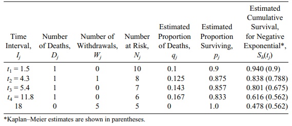
Let us consider the data in Table 15.1 again. There are four events (deaths) at 11.8, 5.4, 1.5, and 4.3 months into the trial and six censored times at 3.2, 12.5, 17.6, 13.3, 15.0, and 13.0 months. The estimate λ_h is just the number of events/total time on test = 4/(11.8 + 5.4 + 1.5 + 4.3 + 3.2 + 12.5 + 17.6 + 13.3 + 15.0 + 13.0) = 4/97.6 = 0.041. So S_h(t) = exp(–0.041t).

Refer to Table 15.4. The column labeled “Estimated Cumulative Survival” com-pares the survival estimates at the event time points, S_h(t_j), for the negative exponential with the results for the Kaplan–Meier (KM) estimates (KM given in parentheses). The discrepancies between the negative exponential and the Kaplan–Meier estimates indicate that the exponential does not fit this model well. The discrepancy is particu-larly noticeable at time 5.4 months, when the parametric estimate is 0.801 and the Kaplan–Meier is 0.675. However, the sample size is small, and this discrepancy may not be statistically significant. Note that for the exponential model the estimates S_h(t_j) = e^–λh^tj. So, since λ_h = 0.041 at t₁ = 1.5, S_h(t₁) = exp[–0.041 (1.5)] = exp(–0.0615) = 0.940. At t₂ = 4.3, S_h(t₂) = exp[–0.041 (4.3)] = exp(–0.1763) = 0.838.

TABLE 15.4. Negative Exponential Survival Estimates for Patients in Table 15.2