Comparing Two or More Survival Curves-The Log Rank Test

COMPARING TWO OR MORE SURVIVAL CURVES-THE LOG RANK TEST

To compare two survival curves in a parametric family of distributions such as the negative exponential or the Weibull, we need to test only the hypothesis that the parameters are equal versus the alternative hypothesis that the parameters differ in some way. We will not go into the details of such parametric comparisons. Howev-er, nonparametric procedures look for differences in survival distributions based on the information in the Kaplan–Meier curves. In this section, we consider specific nonparametric tests for two or more survival curves.

The log rank test, a nonparametric procedure for comparing two or more survival functions, is a test of the null hypothesis that all the survival functions are the same, versus the alternative that at least one survival function differs from the rest. The idea is to compare the observed frequency of deaths or failures for each curve in various time intervals with what would be expected under the null hypothesis that all the curves are the same. Details can be found in the original paper [see Man-tel (1966)] or in Lee (1992), pages 109–112.

Now we will describe a simple chi-square test that is very similar to the log rank test. For the chi-square test, we simply let O₁ be the observed number of deaths in group 1, O₂ the observed number in group 2, O₃ the observed number in group 3, and so on until all the groups have been enumerated.

A chi-square statistic is determined by computing the expected numbers E₁, E₂, E₃, etc., of deaths in each group. For this calculation to hold, all the groups need to come from the same population of survival times. Then, similar to other chi-square calculations (refer to Chapter 11), the statistic χ² = (O₁ – E₁)²/E₁ + (O₂ – E₂)²/E₂ + . . . + (O_k – E_k)²/E_k has approximately a chi-square distribution with k – 1 degrees of freedom when the null hypothesis is true. We will go through an ex-ample in detail in which k = 2, and the test statistic is then chi-square with 1 de-gree of freedom under the null hypothesis.

This simple calculation is taken from Lee (1992), Example 5.2, page 107. Sup-pose that ten female breast cancer patients are randomized to receive either cyclic administration of cyclophosphamide, methatrexate, and fluorouracil (CMF), or no additional treatment after a radical mastectomy. Five patients are randomized to the CMF treatment arm and five to the control arm.

We are interested in knowing whether time to relapse (time in remission) is lengthened by the treatment versus the null hypothesis that the treatment makes no difference. The results at the end of the trial are as follows: CMF patient remission times in months are 23, 16+, 18+, 20+, and 24+; the control group remission times are 15, 18, 19, 19, and 20. The plus sign (+) indicates that the data were right-cen-sored, e.g., 16+ means right-censored at 16 months. The events without plus signs refer to remission, 1 case for the CMF group and all 5 cases for control group.

Table 15.5 shows the remission times (T), the number of remissions at remission time (d₁), the number at risk in group 1 (n_1t), the number at risk in group 2 (n_2t), ex-pected frequency in group 1 (E₁), and expected frequency in group 2 (E₂). We will use these terms to compute a chi-square statistic. In order to complete the table, we list the remission times for the pooled data in ascending order. The remission times ranged from 15 to 23 months.

At each time t, the contribution to E₁ is d_tn_1t/(n_1t + n_2t) and, similarly, for E₂ it is d_tn_2t/(n_1t + n_2t). We know that the observed number of remissions is 1 for group 1 and 5 for group 2. As we see from the first column in the table, the remission times are at times 15, 18, 19, 20, and 23 with two remissions at 19. As described previously, the events without the plus signs are the cases in which the patients relapsed and the time is the time in remission. For the CMF group we saw that the only such event was at 23 months for one patient. For the control group we note that five such events oc-curred at times 15, 18, 19, 19, and 20. So χ² = (O₁ – E₁)²/E₁ + (O₂ – E₂)²/E₂ = (1 – 3.75)²/4.75 + (5 – 2.25)²/2.25 = 1.592 + 3.361 = 4.953. From the chi-square distribu-tion with 1 degree of freedom, we see that this result is statistically significant at the 0.05 level (0.05 > p > 0.01). Note that with 1 degree of freedom the critical value for p = 0.05 is 3.841 and for p = 0.01 it is 6.635. Since 4.953 lies between these values we can conclude that the p-value is between 0.01 and 0.05. Thus, we may conclude that there are significantly shorter remission times in the control group.

Now let’s consider an example from the treatment of prostate cancer. A proce-dure called cryoablation is used to remove tumors from the prostate gland. Re-searchers assigned each patient to one of three risk groups (i.e., risk of recurrence) based on measures of severity of the disease prior to the procedure. Then, the re-searchers followed the patients for up to eight years.

TABLE 15.5. Computation of Expected Numbers for Chi-square Test

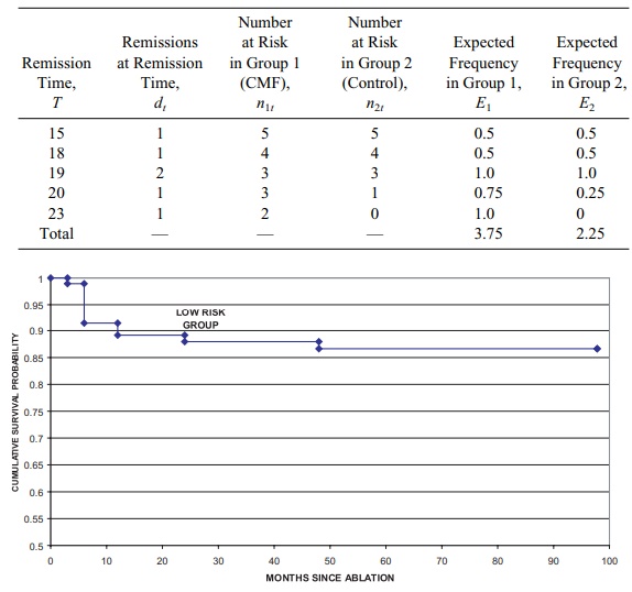
Figure 15.2. Cryoablation biochemical-free survival PSA > 1 criterion.

The three categories of risk were designated as low, moderate, and high. Ka- plan–Meier survival curves were generated for each risk group; the log rank test was used to compare these survival curves. Failure was defined as having a prostate-specific antigen lab test result above 1.0 ng/mL. Figures 15.2, 15.3, and 15.4 present the Kaplan–Meier curves.

The curves are very similar. However, the total sample size was only 561, with 94 patients in the low risk group, 178 in the medium risk group, and 289 in the high-risk group. The p-value for the log rank test was 0.2597, indicating that the curves were not statistically significantly different.

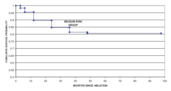
Figure 15.3. Cryoablation biochemical-free survival PSA > 1 criterion.

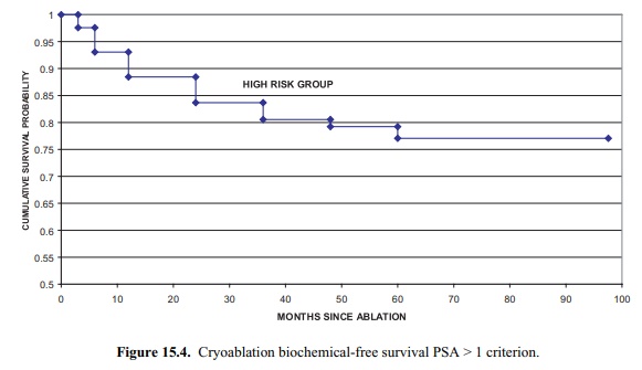
Figure 15.4. Cryoablation biochemical-free survival PSA > 1 criterion.

With this final example, we conclude Chapter 15. You have seen that analyses of survival times yield much useful information regarding the survival of patients and estimation of cure rates. In the next chapter, we will identify computer software programs that can be used for survival analyses. Chapter 16 also will present a vari-ety of software packages that are applicable to many of the statistical techniques covered in this text.