Mean and Standard Deviation for the Binomial Distribution

MEAN AND STANDARD DEVIATION FOR THE BINOMIAL DISTRIBUTION

In Chapter 4, we discussed the mean and variance of a continuous variable (μ, σ² and , S²) for the parameters and their respective sample estimates. It is possible to compute analogs for a dichotomous variable. As shown in Chapter 5, the binomial distribution is used to describe the distribution of dichotomous outcomes such as heads or tails or “successes and failures.” The mean and variance of the binomial distribution are functions of the parameters n and p, where n refers to the number in the population and p to the proportion of successes. This relationship between the parameters n and p and the binomial distribution affects the way we form test statis-tics and confidence intervals for the proportions when using the normal approxima-tion that we will discuss in Section 10.3. The mean of the binomial is np and the variance is np(1 – p), as we will demonstrate.

Recall (see Section 5.7) that for a binomial random variable X with parameters n and p, X can take on the values 0, 1, 2, . . . , n with P{X = k} = C(n, k) p^k(1 – p)^n–k for k = 0, 1, 2, . . . , n. Recall that P{X = k} is the probability of k successes in the n Bernoulli trials and C(n, k) is the number of ways of arranging k successes and n – k failures in the sequence of n trials. From this information we can show with a little algebra that the mean or expected value for X denoted by E(X) is np. This fact is given in Equation 10.1. The proof is demonstrated in Display 10.1 (see page 220).

The algebra becomes a little more complicated than for the proof of E(X) = np shown in Display 10.1; using techniques similar to those employed in the foregoing proof, we can demonstrate that the variance of X, denoted Var(X), satisfies the equation Var(X) = np(1 – p). Equations 10.1 and 10.2 summarize the formulas for the expected value of X and the variance of X.

For a binomial random variable X

E(X) = np                             (10.1)

where n is the number of Bernoulli trials and p is the population success probability. For a binomial random variable X

Var(X) = np(1 – p)               (10.2)

where n is the number of Bernoulli trials and p is the population success probability. To illustrate the use of Equations 10.1 and 10.2, let us use a simple example of a Bernouilli trial in which n = 3 and p = 0.5. An illustration would be an experiment involving three tosses of a fair coin; a head will be called a success. Then the possi-ble number of successes on the three tosses is 0, 1, 2, or 3. Applying Equation 10.1, we find that the mean number of successes is np = 3 (0.5) = 1.5; applying Equation 10.2, we find that the variance of the number of successes is np(1 – p) = 3(0.5)(1 – 0.5) = 1.5(.5) = 0.75. Had we not obtained these two simple formulas by algebra, we could have performed the calculations from the definitions in Chapter 5 (sum-marized in Display 10.1 and Formula D10.1).

To apply Formula D10.1, we compute the probability of each of the successes (outcomes 0, 1, 2, and 3), multiply each of these probabilities by the number of suc-cesses (0, 1, 2, and 3) and then sum the results, as shown in the next paragraph.

The probability of 0 successes is C(3, 0)p⁰(1 – p)³; when we replace p by (0.5), the term C(3, 0)(0.5)⁰(1 – 0.5)³ = (1)(1)(0.5)³ = 0.125. As there are 0 successes,

Display 10.1. Proof that E(X) = np

To conduct this proof, we will use the formula presented in Chapter 5, Section 5.7, in which the probability of r successes in n trials was defined as P(Z = r) = C(n, r)p^r(1 – p)^n–r. For the proof, we replace r by k (the number of trials) and sum over the k trials; this sum equals 1, as shown below:

Σ_kC(n, k)p^k(1 – p)^n–k = 1                           (D10.1)

This equation holds for any positive integer n and proportion 0 < p < 1 when the summation is taken over 0 ≤ k ≤ n. Assume k ≥ 2 for the following argument. The mean denoted by E(X) is by definition

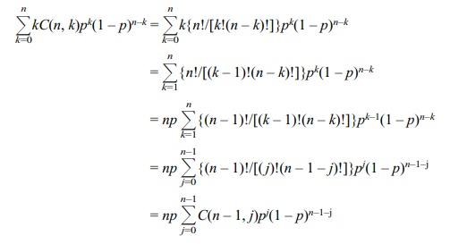
Remember that by applying formula D10.1, with n – 1 in place of n in the formula

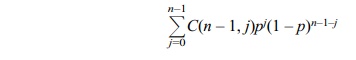
since n – 1 is a positive integer (recall that n ≥ 2, implying that n – 1 ≥ 1). So for n ≥ 2, E(X = np. For n = 1, E(X) = 0(1 – p) + 1(p) = p = np also. So we have shown for any positive integer n, E(X) = np.

we multiply 0.125 by 0 and obtain 0. Consequently, the contribution of 0 suc-cesses to the mean is 0. Next, we calculate the probability of 1 success by using C(3, 1)p(1 – p)², which is the number of ways of arranging 1 success and 2 fail-ures in a row multiplied by the probability of a particular arrangement that has 1 success and 2 failures. C(3, 1) = 3, so the resulting probability is 3p(1 – p)² = 3(0.5)(0.5)² = 3(0.125) = 0.375. We multiply that result by 1, since it corresponds to 1 success and we find that 1 success contributes 0.375 to the mean of the distribution. The probability of 2 successes is C(3, 2)p²(1 – p), which is the number of ways of arranging 2 successes and 1 failure in a row multiplied by the probability of any one such arrangement. C(3, 2) = 3, so the probability is 3p²(1 – p) = 3(0.5)²(0.5) = 0.375. We then multiply 0.375 by 2, as we have 2 successes, which contribute 0.750 to the mean. To obtain the final term, we compute the probabili-ty of 3 successes and then multiply the resulting probability by 3. The probability of 3 successes is C(3, 3) = 1 (since all three places have to be successes, there is only one possible arrangement) multiplied by p³ = (0.5)³ = 0.125. We then multi-ply 0.125 by 3 to obtain the contribution of this term to the mean. In this case the contribution to the mean is 0.375.

In order to obtain the mean of this distribution, we add the four terms together. We obtain the mean = 0 + 0.375 + 0.750 + 0.375 = 1.5. Our long computation agrees with the result from Equation 10.1. For larger values of n and different val-ues of p, the direct calculation is even more tedious and complicated, but Equation 10.1 is simple and easy to perform, a statement that also holds true for the variance calculation. Note that in our present example, if we apply the formula for the vari-ance (Equation 10.2), we obtain a variance of np(1 – p) = 3(0.5)(0.5) = 0.750.