The Mixing of Solids
| Home | | Pharmaceutical Technology |Chapter: Pharmaceutical Engineering: Mixing
Pharmacy offers many important examples of the mixing of solids. In several forms of drug presentation, the attainment of accurate dosage depends on an adequate mixing operation at some stage in production.
THE MIXING OF SOLIDS
Pharmacy
offers many important examples of the mixing of solids. In several forms of
drug presentation, the attainment of accurate dosage depends on an adequate
mixing operation at some stage in production. Since the dose unit may be small,
say 0.1 g, a small scale of scrutiny is applied.
The
mixing of all systems of matter involves a relative displacement of the
particles, whether they are molecules, globules, or small crystals, until a
state of maximum disorder is created and a completely random arrangement is
ach-ieved. Such an arrangement for a mixture of equal parts of two components
is shown in Figure 13.1B.
A
“perfect” mixture, which, with a practical sample, would offer point
uniformity, is shown in Figure 13.1A. Such an arrangement is, however,
virtu-ally impossible, and no mixing equipment can do better than producing the
“random” mixture shown in Figure 13.1B. In such a mixture, the probability of
finding one type of particle at any point in the mixture is equal to the
proportion of that type of particle in the mixture.
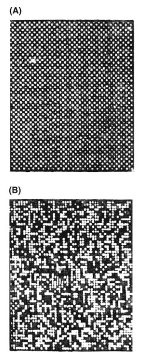
FIGURE 13.1 Diagrammatic representation of (A) a perfect mix and (B) a random mix.
The
mixing of solids differs from the mixing of liquids in that the smallest
practical sample withdrawn from a mixture of two miscible liquids contains many
millions of particles. In the mixing of solids, a small sample contains
relatively few particles, and examination of Figure 13.1B should show that such
samples will show considerable variation with respect to the overall
composi-tion of the mixture and that this variation should be reduced as the
number of particles in the sample is increased. Assessing the variation in,
say, drug content in a series of samples drawn from a mixture of powders is of
great importance. The tablet machine may be regarded as a volumetric sampling
device, and the variation in drug content between one tablet and the next is
largely controlled by the mixing stage that precedes it.
Some Properties of a Random Mixture
“Lacey,
1953” showed that the variation in the composition of samples drawn from a
random mixture of two materials could be expressed by the following relation:
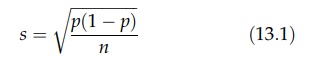
where
s is the standard deviation of the
samples, p is the proportion of one
component, and n is the number of particles in the sample. The relation
requires that the two components are alike in particle size, shape, and density
and can only be distinguished by some neutral property, such as color. If a
very large number of samples, each containing a given number of particles, are
withdrawn from a mixture of equal parts of two materials, the results of
analysis can be presented in the form of a frequency curve in which the samples
are normally distributed around the mean content of the mixture; 99.7% of the
samples will fall within the limits p = 0.5 + 3σ. The standard deviation of the
samples is inversely proportional to the square root of the number of particles
in a sample. If the particle size is reduced so that the same weight of sample
contains four times as many particles, the standard deviation will be halved.
The distribution of samples and the effect of size reduction are shown in
Figure 13.2.
In
a critical examination of pharmaceutical mixing, Train showed that samples of a
random mixture of equal parts of A and B must contain at least 800 particles if
997 out of every 1000 samples (3σ) were to lie between 10% of the
stated composition, that is, the proportion, p, of A = 0.5 ± 0.05, where σ = 0.05/3 (Train, 1960). The effect of
the number of particles in a sample on the percentage variation about the mean
content of a mixture of equal parts A and B was summarized by Train in the
diagram reproduced in Figure 13.3. The diagram may be used to show that if, in
the above example, limits of ±1% were sub-stituted, 90,000 particles must be
present in each sample. The true standard deviation is given by the symbol s. The standard deviation estimated
by the withdrawal of a number of samples is denoted s.
If,
instead of equal parts A and B, the proportion of an active ingredient, A, in
the mixture was 0.1 (10%), imposition of limits of ±10% (in 997 out of 1000
cases) requires that each sample shall contain over 8000 particles. If the
pro-portion of active constituent is 0.01, or 1%, a figure of 90,000 particles
per sample is obtained, and if the limits are reduced to +1%, the active constituent is 0.01,
or 1%, a figure of 90,000 particles per sample is obtained, and if the limits
are reduced to ±1%, the figure is nine million.
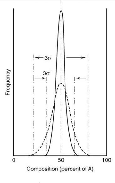
FIGURE 13.2 Distribution of samples drawn
from a mixture of equal parts A and B. The broken line represents data for the
coarser powder.
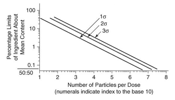
FIGURE 13.3 General theoretical relationship between number of particles and percentage limit of ingredient for a 50:50 mix.
The
theoretical derivation of these results is based on component particles that
are alike in size, shape, and density. This condition is not encountered in the
practical mixing of solids, and, as we shall see later, any of these factors
may prevent the formation of a random mixture. The value of the number of
particles per sample derived in any example must therefore be raised if the
limits given are to be maintained.
As
the proportion of an active ingredient in a mixture decreases, the number of
particles in each sample or dose must increase, and materials of smaller
particle size must be used. This statement indicates the limitation of the
mixing of solids. Production of very fine powders is difficult and often
attended by severe aggregation, thus defeating the object of size reduction in
the mixing process. Where the proportion of active constituent is very small
and is finally presented in a small dose unit, dry mixing of solids may fail to
produce an adequate dispersion of one component in another and other meth-ods,
such as spraying a solution of one component onto another, must then be
adopted.
Another
example of the relation of dose uniformity and number of particles in the dose
is found with two components that are separately granu-lated before mixing.
This procedure is sometimes adopted for reasons of sta-bility during
granulation. The variation in samples drawn from such a system will be much
greater than the variations in a mixture that was mixed before granulation
because the effective number of particles in the sample is greatly reduced.
The Degree of Mixing
A
quantitative expression that defines the state of a mix is necessary if a
rational answer to the question “Is this material well enough mixed?” is to be
made. Such an expression would also allow the course of mixing to be followed
and the performance of different mixers to be compared. The most useful method
of expressing the degree of mixing is by measuring the statistical variation in
composition of a number of samples drawn from the mix. The scale of scrutiny
determines the size of the samples, and their number depends on the accuracy
required of the assessment.
As already shown, a series of samples drawn from a random mix exhibit a standard deviation of sr. An index of mixing, M, suggested by Lacey, is given by
M
= sr/s (13.2)
where
s is the standard deviation of
samples drawn from the mixture under examination (Lacey, 1954). This approaches
unity as mixing is completed. Kramers has suggested that
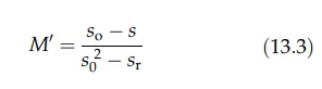
where
so is the standard deviation of samples drawn from the unmixed
mate-rials (Shotton and Ridgway, 1974). It is equal to p(1 - p), where p is the
pro-portion of the component in the mix. Its modification by Lacey, using the
variance of the samples, to
gives
a fundamental equation for expressing the state of the mixture, the index, M”, varying from 0 to 1 (Lacey, 1954).
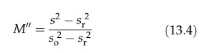
The binomial and Poisson distributions have also been used to examine the state of a mixture. If the proportion of black particles in a random mixture of black and white particles is p, the probability, P(x), of obtaining x black particles in a sample of n particles is given by
If p is small (<0.15) and n is large, the Poisson distribution can be used, when
P(x) = e-m(mx/xl) (13.6)
where m = np, the mean number of black
particles in the samples of n particles. This relation may be used in an
assessment of dry mixing equipment (Adams and Baker, 1956).
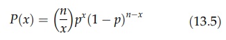
If
m is greater than 20 and more than 10 samples are taken, then
1. about 10 of the
samples will have the number of black particles outside the limits (m ± 1.7H√m),
2. about 5% of the
samples will have the number of black particles outside the limits (m ± 2.0H√m), and
3. about 1% of the
samples will have the number of black particles outside the limits (m ± 2.6H√m).
Results of such
tests in which small cubes of polythene were mixed in a double-cone blender are
shown in Figure 13.4A and B. The probability that the results plotted in Figure
13.4A came from a random mixture is less than 0.01, 19 out of 34 samples
exceeding the 1 in 10 limits. The densities of the two com-ponents in this
example were 0.92 and 1.2. The results given in Figure 13.4B were obtained when
the components were of the same density and the proba-bility that the samples
were drawn from a random mixture was 0.7.
Alternatively,
satisfactory mixing may be established by imposing standards dictated by the
operations in which the mixture is to take part. For example, Kaufman measured
the variance of 10 samples drawn at random from a mixture of procaine
penicillin and dihydrostreptomycin being mixed in a tumbler blender (Kaufman,
1962). The variance of the samples at different times during mixing is shown in
Figure 13.5. The samples, which, in this case, weighed 5 g, represent the
ultimate subdivision of a production-size antibiotic mixture.
FIGURE 13.4 Variation in the number of black
particles in samples drawn from a tumbler blender. (A) p < 0.01 and (B) p =
0.7.
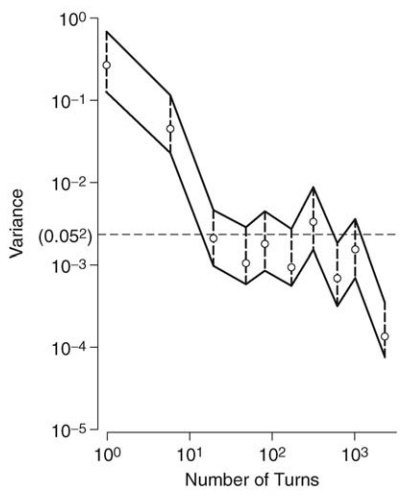
FIGURE 13.5 Decrease in the variance of samples drawn from a mixture of penicillin (40%) and dihydrostreptomycin in a twin-shell blender.
An acceptable degree of
homogeneity was set at a standard deviation of 5%, giving a variance of (0.05)2,
and this was achieved after just over 100 revolutions of the mixer. [The band
around the experimental values of the variance defines the limits within which
the true variance lies (p =
0.9)]. By this method, the suitability of the machine and operating
characteristics were established.
The Mechanism of Mixing and
Demixing
The
randomization of particles by relative movement, one to another, is ach-ieved
by the following mechanisms:
Convective mixing: The transfer of groups of adjacent
particles from one location in the mass to another.
Diffusive mixing: The distribution of particles over a
freshly developing surface.
Shear mixing: The setting up of slip planes
within the mass.
All
take place to some extent during mixing, but they vary in extent with the type
of mixer used. In general, a large diffusional element is necessary if the
scale of scrutiny is small. In addition, distortion of portions of the material
by intense shear forces, as in mulling, and the scattering of individual
particles by impact, processes normally associated with size reduction, are
used for some mixing operations.
Convective
mixing predominates in machines utilizing a mixing element moving in a
stationary container. An example is the horizontal ribbon mixer. Groups of
adjacent particles are moved from one position to another, giving a steady
decrease in the scale of segregation.
Shear
mixing occurs when a system of forces acting on the particles induce the
formation of a slip place. This gives relative displacement of two regions. It
occurs, for example, in the rearrangement of shape as the main charge falls
from end to end in a double-cone mixer. Train has stressed the importance of
expansion or dilation of the material so that shear forces may be effective
(Train, 1960). A practical corollary is that efficiency will be reduced if the
machine is overfilled.
Diffusive
mixing predominates in tumbler mixers. Tumbling occurs as the material is
lifted past its angle of repose. Mixing occurs when a particle changes its path
of circulation through a collision or by being trapped in voids presented by
another layer of particles.
The
mild forces involved in the examples given above may be insufficient to
adequately disperse materials that tend to aggregate. The more energetic
pro-cesses of mulling and impact milling may then be used. Size reduction and
mixing are carried out simultaneously, although the former may be slight. An
example is found in the incorporation of ferric oxide and basic zinc carbonate
in the pro-duction of calamine. For mixing of this type, the hammer mills,
mullers, and ball mills charged with small balls are frequently used. The
material being processed at any time must contain the correct amounts of
materials. If the holdup capacity of the mill is sufficiently large, this can
be achieved by a correctly proportioned feed. Otherwise, the product will have
to be mixed a second time by some other method to correct segregation of large
scale but small intensity.
If
all the particles in a mixture reacted equally to an applied force, then all
mixers would eventually produce a random mixture, although the time taken would
vary, the more efficient mixer producing a random mix more quickly. The
characteristics of real mixtures prevent this, and differences in particle
size, shape, and density oppose randomization. Of these, differences in particle
size are most important. The role of these factors in opposing mixing and
promoting demixing is demonstrated in the analysis of horizontal drum mixing
(Donald and Roseman, 1962). Movement of material in a radial plane is shown in
Figure 13.6. The static mass of particles is lifted past its angle of repose,
and particles tumble down the free surface, accelerating to the center of the
mixer and then decelerating before entering the static bed. The zone in which
this takes place is the mixing zone, and since it is in contact with the static
bed, in which no mixing takes place and which is moving in the opposite
direction, a velocity gradient occurs across the mixing zone, that is, a layer
of particles is passing over the layer beneath, and so on. This zone is in an
expanded state, and particles are
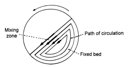
FIGURE 13.6 The mechanism of radial mixing
and demixing.
Mixing occurs when a particle is
trapped by moving into a void, thus changing its path of circulation. This
mechanism suggests an optimum running speed. If it is too slow, not enough
events occur. If it is too fast, there is not sufficient time for capture.
As
long as one type of particle is not preferentially caught, a random mix will
eventually occur in the radial plane. If, however, one component is smaller or
denser or has certain shape characteristics, it will be preferentially trapped
and will move into the lower layers of the mixing zone until it finally
concen-trates as a central core running the length of the mixer. Similar
effects occur in axial mixing, and the final shape of the segregated zone
formed under the influence of axial and radial movements depends on the flow
properties of the material. Similar effects have been reported with a
double-cone blender (Adams and Baker, 1956). Segregation will also occur with
such materials when they are dumped from the mixer.
In
general, one component will concentrate at one position in the mixer when a
simple, repetitive, and symmetric movement occurs. Modern design tends to the
rotation of asymmetric shapes or to symmetric shapes rotated asymmetrically,
often with an abrupt reversal in the movement of the charge. Even so,
segregation may still occur after a long period of mixing. The variance of
samples decreases during mixing to a minimum value. This is followed by a
period of demixing, the variance finally achieving a higher equilibrium value.
It is therefore possible to overmix.
The Rate of Mixing
Since mixing is a process of achieving uniform randomness, the rate of mixing is proportional to the amount of mixing still to be done. If, at the start of mixing, a particle changes its path of circulation, it is most likely to find itself in a different environment. The rate of mixing is therefore fast. At the end of the process, the particle is less likely to find a different environment, and such a change gives no useful mixing. Fewer mixing events will take place, and the rate of mixing finally reaches zero. The rate of mixing for any mixing mechanism can be rep-resented by the following expression:
dM/dt = k(1 – M) (13.7)
where M, the index of mixing, has already been defined. Integration of this equation gives
M = 1 – e-kt (13.8)
The
rate constant, k, depends on the
physical nature of the materials being mixed and on the geometry and operation
of the mixer.
