Understanding Chi-Square

UNDERSTANDING CHI-SQUARE

In chapters 8 and 9, we covered the t test and Z test, which use interval or ratio mea-sures. Now we turn to the chi-square test, which is appropriate for nominal and or-dinal measurement. The chi-square test may be used for two specific applications: (1) to assess whether an observed proportion agrees with expectations; (2) to deter-mine whether there is a statistically significant association between two variables (such as variables that represent nominal level measurement or, in some cases, ordi-nal level measurement).

In the case of testing the association between two or more variables, the data are portrayed as contingency tables. these tables are also known as cross-tabulation ta-bles. For example, the investigator might cross-tabulate the results for a study of gender and smoking status. A chi-square test could be used to determine the associ-ation between these two variables. Later, we will give an example of how to set up a contingency table and perform a chi-square test.

The formula for many test statistics with approximate chi-square distributions is:

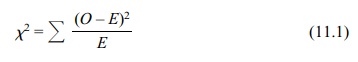
where

O = observed frequency

E = expected frequency

As an example of one of the simplest uses of the foregoing formula, let us per-form the chi-square test for a single proportion. (We will see that in some instances, the chi-square test may be used as an alternative to tests of proportion discussed in Chapter 10.) The chi-square test that we will use in this example shall be called a test with an a priori theoretical hypothesis, because the expected frequency of the outcome is known theoretically.

Suppose we run a coin toss experiment with 100 trials and find 70 heads; is this a biased outcome? That is, we want to know whether this is a very unusual event for a fair coin toss. If so, we may decide that the alternative—that the coin is loaded in favor of heads—may be more plausible. The data may be portrayed as shown in Table 11.1.

We would expect a fair coin toss to produce 50% heads and 50% tails in the long run (the theoretical a priori expectation). Table 11.1 lists all of the elements required by the chi-square formula to calculate the chi-square statistic. 

TABLE 11.1. Data from a Coin Toss Experiment

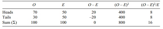
This value is shown at the intersection of the last column and last row. Substituting it in the chi-square formula, we obtain:

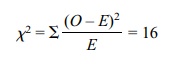
In order to evaluate whether this is a significant chi-square value—i.e., whether the coin toss is unfair—we need to compare the result we have obtained with the value in a chi-square table. We need to know the number of degrees of freedom as-sociated with the coin toss experiment. Degrees of freedom (the term means “free to vary”) are denoted by the symbol df. In this case, df = 1. (You may surmise that in a given number of coin tosses, once the number of heads is known, then the number of tails is fixed; only one value is free to vary. Let us say that in a small trial of 10 coin tosses, we find six heads; the number of tails must be four.)

In our example, we need to do a table lookup to determine the chi-square critical value. As with other statistical tests, the level of significance may be set to p < 0.05 or 0.01 or 0.001. We know from a chi-square table that the chi-square critical value is 3.84 for df = 1 at p < 0.05.

Therefore, the null hypothesis that the coin toss is unbiased would be rejected, as we obtained a chi-square of 16. The coin toss seems to be favoring heads. By the way, it is helpful to memorize this particular chi-square value as it comes up in many situations that have one degree of freedom, such as the 2 × 2 tables (shown in Sections 11.3 and 11.6).

One of the best statistical texts that deals explicitly with categorical data is Agresti (1990). Refer to it if you are interested in more details or aspects of the theory.