Testing Independence between Two Variables

TESTING INDEPENDENCE BETWEEN TWO VARIABLES

In testing independence between two variables, we do not assume an a priori expected outcome or theoretical (alternative) hypothesis. For example, we might want to know whether men differ from women in their preference for Western medicine or alternative medicine for treatment of stress-related medical problems. 

TABLE 11.2. Gender and Preference for Medical Care

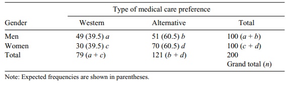
In this example, we assume that subjects can select only a single preference such as Western or alternative, but not both types. Our null hypothesis will be that the proportions in each category do not differ. There are a total of 200 subjects, equally divided be-tween men and women as shown in Table 11.2; this is called a contingency table or cross-tabulation of two variables.

The table presents the observed frequencies from a survey of a research sample. Now we need to compute the expected frequencies for each of the four cells. This calculation uses the formula [(a + b)(a + c)]/n for cell a. The formula is based on the null hypothesis that assumes no difference between men and women. This is the same as saying that the rows and columns are statistically independent. So the ex-pected proportion of men who prefer Western medicine should be the population total n multiplied by the probability of being a man preferring Western medicine. The probability of being a man is estimated by the frequency (a + b)/n, the propor-tion of men in the table (sample). The probability of preferring Western medicine is estimated by (a + c)/n, the proportion of people favoring Western medicine in the table. The independence assumption lead to multiplication of these two probabili-ties, namely [(a + b)/n] [(a + c)/n] or (a + b)(a + c)/n². The foregoing formula is then obtained in a manner similar to that for an expectation for a binomial total; i.e., np, where in this case p = (a + b)(a + c)/n². So the expected total for the cell is n{(a + b)(a + c)/n²} = (a + b)(a + c)/n. This same idea can be applied to obtain the ex-pectations for the other three cells.

To calculate the expected frequency for cell a, we first determine the proportion of males and females (100/200 = 0.5) and then multiply this result by the respective column totals (e.g., the expected frequency for men who prefer Western medicine is 0.5 × 79 = (39.5) The general formula for the expected frequency in each cell is as follows:

E(a) = [(a + b)/n](a + c) =  (a + b)(a + c) / n

E(b) = [(a + b)/n](b + d) = (a + b)(b + d) / n

E(c) = [(c + d)/n](a + c) = (c + d)(a + c) / n

E(d) = [(c + d)/n](b + d) = (c + d)(b + d) / n

chi-square = (49 – 39.5)²/39.5 +  (30 – 39.5)²/39.5 + (51 – 60.5)²/60.5 + (70 – 60.5)²/60.5 = 7.55

where df = 1, χ² critical value = 3.84, and α = 0.05. In contingency tables, degrees of freedom (df) = (# rows – 1)( # columns – 1). For example, in this table, the chi-square critical value = 3.84, a = 0.05, df = 1 [df = (r – 1)(k – 1) = 1]. We have obtained chi-square = 7.55, which exceeds the critical value. The result is statistically significant, suggesting that there are gender differences in preference for alternative medicine treatments for stress-related illnesses.

Now, in the next example (refer to Table 11.3), we will consider a chi-square test for a table that has more than two columns or rows. This type of table is called an r x c contingency table because there can be r rows and c columns. We will limit our example to a 3 × 3 table, i.e., one that has three rows and three columns. By exten-sion, it will be possible to apply this example to tables that have r and c rows and columns.

Each cell in the contingency table is given an “address” depending on where it is located. Note that the first cell is n_1,1. The first subscripted number refers to the row and the second to the column; the last cell is n_3,3. The notations for the respective row and column totals are shown in the table.

The expected frequencies are computed as follows:

E(n_1,1) = (Σn₁.)( Σn_.1 ) / n

E(n_2,1) = (Σn₂.)( Σn_.1 ) / n

E(n_3,3) = (Σn₃.)( Σn_.3 ) / n

There may be delays in participating in breast cancer screening programs ac-cording to racial group membership. As a result, some racial groups may tend to present with more advanced forms of breast cancer. Data from a hypothetical breast cancer staging study are shown in Table 11.4. We wish to test the hypothesis that

TABLE 11.3. Notation Used in a 3 × 3 Contingency Table

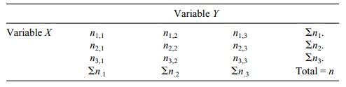
TABLE 11.4. Computation Example—the Association between Race/Ethnicity and Breast Cancer Stage in a Sample of Tumor Registry Patients

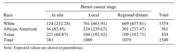
the proportions of each racial classification by stage of breast cancer are equal. The expected frequencies shown in parentheses in Table 11.4 have been computed by using the foregoing formulas. For example, cell (1, 1): (1554 × 381)/2549 = 232.2770. Then we compute (O – E) ²/E. These values are reported in Table 11.5.

Referring to Table 11.5, you can see that chi-square is 552.0993. The degrees of freedom are (r – 1)(c – 1) = (3 – 1)(3 – 1) = 4. At the 0.001 level, a chi-square value of 16.266 would be statistically significant. Thus, we may conclude that cancer di-agnoses are not equally distributed by proportion across the contingency table.