Goodness of Fit Tests-Fitting Hypothesized Probability Distributions

GOODNESS OF FIT TESTS-FITTING HYPOTHESIZED PROBABILITY DISTRIBUTIONS

Goodness of fit tests are tests that compare a parametric distribution to observed data. Tests such as the Kolmogorov–Smirnov test look at how far a parametric cumulative distribution (e.g., normal or negative exponential) deviates from the em-pirical distribution. There is a chi-square test for goodness of fit. Recall the negative exponential distribution is a distribution with the probability density f(x) = λ exp(–λx) for x > 0, where λ > 0 is known as the rate parameter.

For the chi-square test, we divide the range of possible values for a random vari-able into connected disjoint intervals. By this we mean that if the random variable can only take on values in the interval [0, 10] then the set of disjoint connected in-tervals could be [0, 2), [2, 4), [4, 6), [6, 8), and [8, 10]. These intervals are disjoint because they contain no points in common. They are connected because there are no points missing in between the intervals and when they are put together they com-prise the entire range of possible values for the random variable.

For each interval, we count the number (or proportion) of observations from the observed data that fall in that interval. We also compute an expected number for the fitted probability distribution. The fitted probability distribution is simply the para-metric distribution that uses estimates for the parameters in place of the unknown parameters. For example, a fitted normal distribution would use the sample mean and sample variance in place of the parameters μ and σ², respectively. As with the other chi-square tests described in this chapter, we compute the quantities (O_i – E_i)²/E_i for each interval i and sum them up over all the intervals i = 1, 2, . . . , k. Here E_i is obtained by integrating the fitted probability density function over the ith interval.

Under the null hypothesis that the data come from the parametric distribution, the test statistic has an approximate chi-square distribution with k – q – 1 degrees of freedom, where q is the number of parameters estimated from the data to compute the expected values E_i.

So for a normal distribution, we would need to estimate the mean and standard deviation. Consequently, q would be 2 and the degrees of freedom would be k – 3. For a negative exponential distribution, we need to estimate only the rate parameter, so q = 1 and the degrees of freedom are k – 2. Recall that the rate parameter mea-sures how many events we expect per unit time. Generally, we do not know its val-ue a priori but can estimate it after the data have been collected. For a detailed ac-count of goodness of fit tests for both continuous and discrete random variables, see the Encyclopedia of Statistical Sciences, Volume 3 (1983), pp. 451–461.

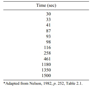
The following example, taken from Nelson (1982), represents complete lifetime data for a negative exponential model. The table presents the time to breakdown of insulating fluid at a voltage of 35 kV. In this case, we have 12 observed times, which are shown in Table 11.14.

TABLE 11.14. Seconds to Insulating Fluid Breakdown at 35 kV*

First, we need to estimate the rate parameter. The best estimate of expected time to failure is the sum of the failure times divided by the number of failures. This esti-mate is often referred to as the mean time between failures. Using the data in Table 11.14, we calculate the mean time between failures as follows:

(30 + 33 + 41 + 87 + 93 + 98 + 116 + 258 + 461 + 1180 + 1350 + 1500)/12 = 437.25 seconds

The reciprocal of this quantity is called the failure rate. In our example, it is 0.002287 failures per second.

Now we can determine for any interval the probability of failure in the interval denoted p_i for interval i. Since S(t) = exp(–λt) is the survival probability for the interval [0, t], we can estimate λ as 0.002287. For any interval, i = [a_i, b_i], and p_i, the probability of failure in interval i, is estimated as exp(–0.002287a_i) – exp(–0.00287b_i).

Suppose we have a range of values [0,∞]. Now let us divide [0,∞] into four dis-joint intervals: [0, 90], [90, 180], [180, 500], and [500,∞]. We observe four failures in the first interval, two failures in the second interval, two failures in the third in-terval, and three in the last interval. For each i, E_i = np_i. The resulting computations for this case, where n = 12, are given in Table 11.15.

In this example, the chi-square statistic is 2.13. We refer to the chi-square table (Appendix D) for the distribution under the null hypothesis. Since k = 4 and q = 1, the degrees of freedom are k – q – 1 = 2. From Appendix D we see that the p-value is between 0.10 and 0.90. So we cannot reject the null hypothesis of a negative exponential distribution. The data seem to fit the negative exponential distribution reasonably well.