Exercises questions answers

EXERCISES

11.1 State in your words definitions of the following terms:

a.     Chi-square

b.     Contingency table (cross-tabulation)

c.      Correlated proportions

d.     Odds ratio

e.      Goodness of fit test

f.       Test for independence of two variables

g.     Homogeneity

11.2 A hospital accrediting agency reported that the survival rate for patients who had coronary bypass surgery in tertiary care centers was 93%. A sample of community hospitals had an average survival rate of 88%. Were the survival rates for the two types of hospitals the same or different?

11.3 Researchers at an academic medical center performed a clinical trial to study the effectiveness of a new medication to lower blood sugar. Diabetic patients were assigned at random to treatment and control conditions. Patients in both groups received counseling regarding exercise and weight loss. 

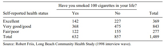
TABLE 11.16. Cross-Tabulation of Lifetime Smoking and Self-Reported Health Status

Among the sample of 200 treatment patients, 60% were found to have normal fasting blood glucose levels at follow-up. Among an equal number of controls, only 15% had normal fasting blood glucose levels at follow-up. Demonstrate that the new medication was effective in treating hyperglycemia.

11.4 In a community health survey, individuals were randomly selected for partic-ipation in a telephone interview. The study used a cross-sectional design. Table 11.16 shows the results for the cross-tabulation of cigarette smoking and health status. Determine whether the relationship between smoking 100 cigarettes during one’s life and self-reported health status is statistically sig-nificant at the a = 0.05 level.

11.5 In the community health survey described in the previous exercise, respon-dents’ smoking status was classified into three categories (smoker, quitter, never smoker). Table 11.17 shows the results for the cross-tabulation of smoking status and health status. Determine whether the relationship is statis-tically significant at the α = 0.05 level. Compare your results with those ob-tained in the previous exercise.

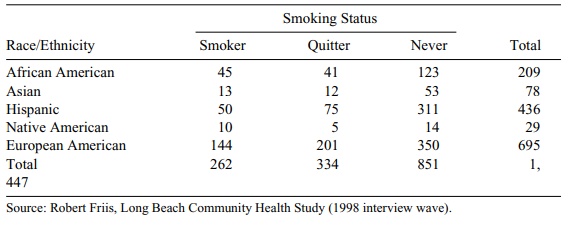
11.6 In the same community health survey, the investigators wanted to know whether smoking status varied according to race/ethnicity. Race was mea-sured according to five categories (African American, Asian, Hispanic, Native American, European American) and smoking status was classified ac-cording to the same categories as in Exercise 11.6. Table 11.18 shows the re-sults for the cross-tabulation of race and health status. Does smoking status vary according to race? Perform the test at the α = 0.05 level.

TABLE 11.17. Cross-Tabulation of Smoking Status and Self-Reported Health Status

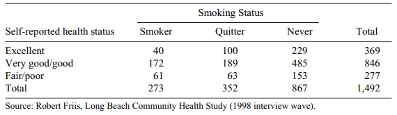
TABLE 11.18. Cross-Tabulation of Race/Ethnicity and Self-Reported Health Status

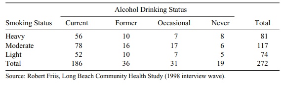
11.7 In the community health survey, the investigators studied the relationship be-tween alcohol drinking status (defined according to four categories) and smok-ing status (defined according to three categories). Alcohol drinking status was classified according to the categories of current drinker, former drinker, occasional drinker, and never drinker. Table 11.19 shows the resulting cross-tabulation. Inspect the data shown in the table. Do you think that there is an association between alcohol drinking status and smoking status? Confirm your subjective impressions by performing a statistical test at the α = 0.05 level.

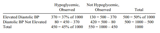
11.8 A multiphasic health examination was administered to 1000 employees of a pharmaceutical firm. 50% of these employees had elevated diastolic blood pressure and 45% had hypoglycemia. A total of 37% of employees had both elevated diastolic blood pressure and hyperglycemia. Create a 2 × 2 contingency table and fill in all cells of the table. Is the association between hyper-tension and hyperglycemia statistically significant?

TABLE 11.19. Cross-Tabulation of Smoking Status and Alcohol Drinking Status

Answers:

11.3

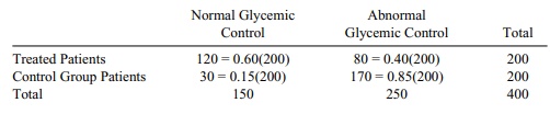
Yes if the treatment was ineffective we would see independence in the 2 × 2 table and approximatelyonly approximately 37.5% or 75 students would have normal control in each group. We would expect 37.5% or about 75 to be normal on one test and the same 75 on the other. So the expected table would be as follows:

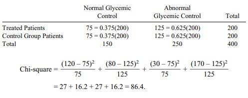
Chi-square = (120 – 75)² / 75 + (80 – 125)² / 125 + (30 – 75)² / 75 + (170 – 125)² / 125

= 27 + 16.2 + 27 + 16.2 = 86.4.

Since we are looking at a chi-square statistic with 1 degree of freedom, we should clearly reject independence in favor of the conclusion that the treatment is effective.

11.4 We recall that the chi-square test applies to testing independence between two groups. The expected frequencies are the row total times the column total di-vided by the total sample size. So in the survey, the participants’ health as self-re-ported versus having smoked 100 or more cigarettes or not in their lifetime should have about the same distribution in each column. So in the first row, for example, E = 632(369)/1489 = 156.62 for the participants who smoked 100 or more cigarettes and E = 857(369)/1489 = 212.38 for those that smoked less than 100 cigarettes. Continuing in this way the table looks as follows:

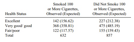
Summing (O – E)²/E we get 1.36 + 1.01 + 0.026 + 0.214 + 0.167 + 0.123 = 2.9. Since this table has 3 rows and 2 columns, the degrees of freedom for the chi-square is (R – 1)(C – 1) = 2(1) = 2. Checking the 5% critical value in the chi-square table, we see that C = 5.991, and since 2.9 < 5.991, we cannot reject the null hypothesis that the distribution of health status for is the same for those that smoked 100 or more cigarettes compared with those that did not smoke 100 or more cigarettes. Al-though it may be surprising that the distributions are so similar, it only indicates that they perceive their health similarly. Their actual health status by other measures could be considerably different.

11.7 The approach is the same as in 11.4 except that R = 2 and C = 2. So the chi-square statistic will have only 1 degree of freedom. First we must construct the table as follows:

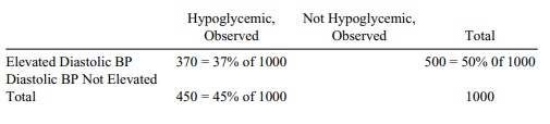
This is what we are given for the table. We can fill in the remaining cells by sub-traction since we know the totals for the first row, the first column, and the grand total:

Now we compute the expected numbers and compute the chi-square statistic:

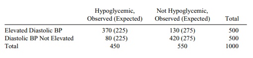
Inspection of the table shows a very poor fit. Computing chi-square we have (145)²/225 + (145)²/275 + (145)²/225 + (145)²/275 = 93.44 + 76.45 + 93.44 + 76.45 = 339.79. The critical value at the 1% level for a chi-square with 1 degree of freedom is C = 6.635. So clearly we reject the null hypothesis. There is a strong relationship between elevated diastolic blood pressure and hypoglycemia for this population.