Logistic Regression
| Home | | Advanced Mathematics |Chapter: Biostatistics for the Health Sciences: Correlation, Linear Regression, and Logistic Regression
Logistic regression is a method for predicting binary outcomes on the basis of one or more predictor variables (covariates).
LOGISTIC REGRESSION
Logistic regression is a method for predicting
binary outcomes on the basis of one or more predictor variables (covariates).
The goal of logistic regression is the same as the goal of ordinary multiple
linear regression; we attempt to construct a model to best describe the
relationship between a response variable and one or more inde-pendent
explanatory variables (also called predictor variables or covariates). Just as
in ordinary linear regression, the form of the model is linear with respect to
the re-gression parameters (coefficients). The only difference that
distinguishes logistic regression from ordinary linear regression is the fact
that in logistic regression the response variable is binary (also called
dichotomous), whereas in ordinary linear re-gression it is continuous.
A dichotomous response variable requires that we
use a methodology that is very different from the one employed in ordinary
linear regression. Hosmer and Lemeshow (2000) wrote a text devoted entirely to
the methodology and many im-portant applications of handling dichotomous
response variables in logistic regres-sion equations. The same authors cover
the difficult but very important practical problem of model building where a
“best” subset of possible predictor variables is to be selected based on data.
For more information, consult Hosmer and Lemeshow (2000).
In this section, we will present a simple example
along with its solution. Given that the response variable Y is binary, we will describe it as a random variable that takes on
either the value 0 or the value 1. In a simple logistic regression equation
with one predictor variable, X, we
denote by π(x) the probability that the response
variable Y equals 1 given that X = x.
Since Y takes on only the values 0
and 1, this probability π(x) also is equal to E(Y|X = x) since E(Y|X
= x) = 0 P(Y = 0|X = x) + 1 P(Y
= 1|X = x) = P(Y = 1|X = x) = π(x).
Just as in simple linear regression, the regression
function for logistic regression is the expected value of the response
variable, given that the predictor variable X
= x. As in ordinary linear regression
we express this function by a linear relationship of the coefficients applied to the predictor variables. The linear
relationship is spec-ified after making a transformation. If X is continuous, in general X can take on all values in the range (–∞`, +∞`).
However, Y is a dichotomy and can be
only 0 or 1. The expectation for Y,
given X = x, is that π(x) can belong only to [0, 1]. A linear combination
such as α + βx can be in (–∞`, +∞`) for continuous variables. So we con-sider the
logit transformation, namely g(x) = ln[π(x)/(1 – π(x)]. Here the transfor-mation w(x) = [π(x)/(1 – π(x)] can take a value from [0, 1] to [0, +`) and ln (the logarithm to the base e)
takes w(x) to (–∞`, +∞`). So this logit transformation puts g(x)
in the same interval as α + βx for
arbitrary values of α and β.
The logistic regression model is then expressed
simply as g(x) = α + βx where g is
the logit transform of π. Another way to express this relationship is on a probability scale by
reversing (taking the inverse) the transformations, which gives π(x) = exp(α + βx)/[1 + exp(α + βx)], where exp is the exponential function. This is
because the exponential is the inverse of the function ln. That means that
exp(ln(x)) = x. So exp[g(x)] = exp(α + βx) = exp{ln[π(x)/(1 – π(x)]} = π(x)/1 – π(x). We then solve exp(α + βx) = π(x)/1 – π(x) for π(x) and get π(x) = exp(α + βx)[1 – π(x)] = exp(α + βx) – exp(α + βx)π(x). After moving exp(α + βx) π(x) to the other side of the equation, we have π(x) + exp(α + βx)π(x) = exp(α + βx) or π(x)[1 + exp(α + βx)] = exp(α + βx). Dividing both sides of the equation by 1 + exp(α + βx) at last gives us π(x) = exp(α + βx)/[1 + exp(α + βx)].
The aim of logistic regression is to find estimates
of the parameters α and β that best fit an available set of data. In ordinary
linear regression, we based this estima-tion on the assumption that the
conditional distribution of Y given X = x
was nor-mal. Here we cannot make that assumption, as Y is binary and the error term for Y given X = x takes on one of only two values, –π(x) when Y = 0 and 1 – π(x) when Y = 1 with probabilities
1 – π(x) and π(x), respectively. The error term has mean zero and
variance [1 – π(x)]π(x). Thus, the error term is just a Bernoulli random
variable shifted down by π(x).
The least squares solution was used in ordinary
linear regression under the usual assumption of constant variance. In the case
of ordinary linear regression, we were told that the maximum likelihood
solution was the same as the least squares solu-tion [Draper and Smith (1998),
page 137, and discussed in Sections 12.8 and 12.10 above]. Because the
distribution of error terms is much different for logistic regres-sion than for
ordinary linear regression, the least squares solution no longer applies; we
can follow the principle of maximizing the likelihood to obtain a sensible
solu-tion. Given a set of data (yi,
xi) where i = 1, 2, . . . , n and the yi
are the observed re-sponses and can have a value of either 0 or 1, and the xi are the corresponding
co-variate values, we define the likelihood function as follows:
L(x1, y1, x2, y2,
. . . , xn, yn) = π(x1)y1[1 – π(x1)](1–y1) π(x2)y2[1 – π (x2)](1–y2) π(x3)y3[1 – π(xn)](1–y3), . . . , π(xn)yn[1 – π(xn)](1–yn) (12.1)
This formula specifies that if yi = 0, then the probability that yi = 0 is 1 – π(xi); whereas, if yi
= 1, then the probability of yi
= 1 is π(xi). The expression π(xi)yi[1
– π(xi)](1–yi) provides
a compact way of expressing the probabilities for yi = 0 or yi = 1 for each i
regardless of the value of y. These
terms shown on the right side of the equal sign of Equation 12.8 are multiplied
in the likelihood equation because the observed data are assumed to be
independent. To find the maximum values of the likelihood we solve for α and β
by simply computing their partial derivatives and setting them equal to zero. This
computation leads to the likelihood equations Σ[yi – π(xi)] = 0 and Σxi[yi – π(xi)] = 0 which we solve simultaneously for α and β. Recall that in the likelihood equations π(xi) = exp(α + βxi)/[1 + exp(α + βxi)], so the parameters α and β enter the likelihood equations through the
terms with π(xi).
Generalized linear models are linear models for a
function g(x). The function g is
called the link function. Logistic regression is a special case where the logit
func-tion is the link function. See Hosmer and Lemeshow (2000) and McCullagh
and Nelder (1989) for more details.
Iterative numerical algorithms for generalized
linear models are required to solve maximum likelihood equations. Software
packages for generalized linear models provide solutions to the complex
equations required for logistic regression analysis. These programs allow you
to do the same things we did with ordinary sim-ple linear regression—namely, to
test hypotheses about the coefficients (e.g., whether or not they are zero) or
to construct confidence intervals for the coeffi-cients. In many applications,
we are interested only in the predicted values π(x) for
given values of x.
Table 12.10 reproduces data from Campbell and
Machin (1999) regarding he-moglobin levels among menopausal and nonmenopausal
women. We use these data in order to illustrate logistic regression analysis.
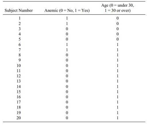
Campbell and Machin used the data presented in
Table 12.10 to construct a lo-gistic regression model, which addressed the risk
of anemia among women who were younger than 30. Female patients who had
hemoglobin levels below 12 g/dl were categorized as anemic. The present authors
(Chernick and Friis) dichotomized the subjects into anemic and nonanemic in
order to examine the relationship of age (under and over 30 years of age) to
anemia. (Refer to Table 12.11.)
We note from the data that two out of the five
women under 30 years of age were anemic, while only two out of 15 women over 30
were anemic. None of the women who were experiencing menopause was anemic. Due
to blood and hemoglobin loss during menstruation, younger, nonmenopausal women
(in comparison to menopausal women) were hypothesized to be at higher risk for
anemia.
In fitting a logistic regression model for anemia
as a function of the di-chotomized age variable, Campbell and Machin found that
the estimate of the re-gression parameter β was 1.4663 with a standard error of 1.1875. The Wald test, analogous to
the t test for the significance of a
regression coefficient in ordinary lin-ear regression, is used in logistic
regression. It also evaluates whether the logistic
TABLE 12.10. Hemoglobin Level (Hb), Packed Cell Volume (PCV), Age, and
Menopausal Status for 20 Women*
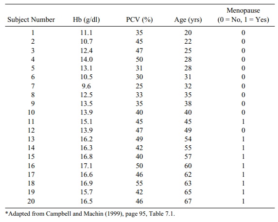
TABLE 12.11. Women Reclassified by Age Group and Anemia (Using Data from
Table 12.10)
With such a small sample size (n = 20) and the dichotomization used, one cannot find a statistically
significant relationship between younger age and anemia. We can also examine
the exponential of the parameter estimate. This exponential is the estimated
odds ratio (OR), defined elsewhere in this book. The OR turns out to be 4.33,
but the confidence interval is very wide and contains 0.
Had we performed the logistic regression using the
actual age instead of the dichotomous values, we would have obtained a
coefficient of –0.2077 with a standard error of 0.1223 for the regression
parameter, indicating a decreasing risk of anemia with increasing age. In this
case, the Wald statistic is 2.8837 (p
= 0.0895), indicating that the downward trend is statistically significant at
the 10% level even for this relatively small sample.
Related Topics
