Regression Analysis and Least Squares Inference Regarding the Slope and Intercept of a Regression Line

REGRESSION ANALYSIS AND LEAST SQUARES INFERENCE REGARDING THE SLOPE AND INTERCEPT OF A REGRESSION LINE

We will first consider methods for regression analysis and then relate the concept of regression analysis to testing hypotheses about the significance of a regression line.

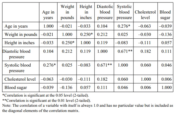
TABLE 12.4. Matrix of Pearson Correlations among Coronary Heart Disease Risk Factors, Men Aged 57–97 Years (n = 70)

The method of least squares provides the underpinnings for regression analysis. In order to illustrate regression analysis, we present the simplified scatter plot of six observations in Figure 12.3.

The figure shows a line of best linear fit, which is the only straight line that minimizes the sum of squared deviations from each point to the regression line. The deviations are formed by subtending a line that is parallel to the Y axis from each point to the regression line. Remember that each point in the scatter plot is formed from measurement pairs (x, y values) that correspond to the abscissa and ordinate. Let Y correspond to a point on the line of best fit that corresponds to a particular y measurement. Then Y – Yˆ = the deviations of each observed ordinate from Y, and

From algebra, we know that the general form of an equation for a straight line is: Y = α + βx, where a = the intercept (point where the line crosses the ordinate) and b = the slope of the line. The general form of the equation Y = α + βx assumes Cartesian coordinates and the data points do not deviate from a straight line. In regression analysis, we need to find the line of best fit through a scatterplot of (X, Y) measurements. Thus, the straight-line equation is modified somewhat to allow for error between observed and predicted values for Y. 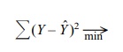The model for the regression equation is Y = α + βx + e, where e denotes an error (or residual) term that is estimated by Y – Y ˆ and Σ(Y – ˆY )² = Σe² . The prediction equation for Yˆ is Yˆ = α + βx.

The term Y ˆ is called the expected value of Y for X. Y ˆ is also called the conditional mean. The prediction equation Yˆ = α + βx is called the estimated regression equation for Y on X. From the equation for a straight line, we will be able to estimate (or predict) a value for Y if we are given a value for X. If we had the slope and intercept for Figure 12.2, we could predict systolic blood pressure if we knew only a subject’s diastolic blood pressure. The slope (b) tells us how steeply the line in-clines; for example, a flat line has a slope equal to 0.

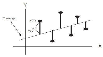
Figure 12.3. Scatter plot of six observations.

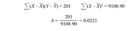
Substituting for Y in the sums of squares about the regression line gives Σ(Y – Y ˆ )² = Σ(Y – a – bX)². We will not carry out the proof. However, solving for b, it can be demonstrated that the slope is

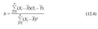
Note the similarity between this formula and the deviation score formula for r shown in Section 12.4. The equation for a correlation coefficient is

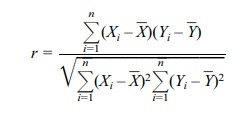
This equation contains the term Σⁿ_i=1(Y_i – )² in the denominator whereas the formu-la for the regression equation does not. Using the formula for sample variance, we may define

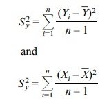
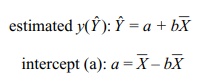
The terms s_y and s_x are simply the square roots of these respective terms. Alternatively, b = (S_y/S_x)r. The formulas for estimated y and the y-intercept are:

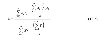
In some instances, it may be easier to use the calculation formula for a slope, as shown in Equation 12.5:

In the following examples, we will demonstrate sample calculations using both the deviation and calculation formulas. From Table 12.2 (deviation score method):

From Table 12.3 (calculation formula method):

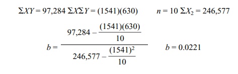
Thus, both formulas yield exactly the same values for the slope. Solving for the y-intercept (a), a = Y –  = 63 – (0.0221)(154.10) = 59.5944.

The regression equation becomes Y ˆ = 59.5944 + 0.0221x or, alternatively, height = 59.5944 + 0.0221 weight. For a weight of 110 pounds we would expect height = 59.5944 + 0.0221(110) = 62.02 inches.

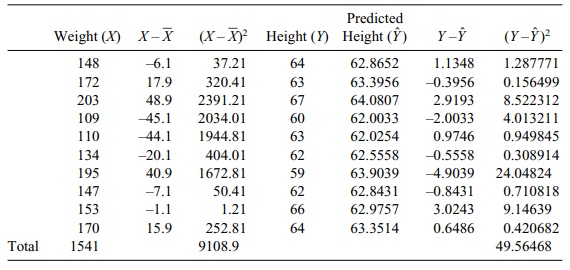
We may also make statistical inferences about the specific height estimate that we have obtained. This process will require several additional calculations, includ-ing finding differences between observed and predicted values for Y, which are shown in Table 12.5.

We may use the information in Table 12.5 to determine the standard error of the estimate of a regression coefficient, which is used for calculation of a confidence interval about an estimated value of Y(Y ˆ). Here the problem is to derive a confidence interval about a single point estimate that we have made for Y. 

TABLE 12.5. Calculations for Inferences about Predicted Y and Slope

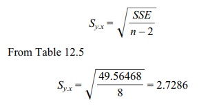
The calculations involve the sum of squares for error (SSE), the standard error of the estimate (s_y,x), and the standard error of the expected Y for a given value of x [SE(Y ˆ)]. The respective formulas for the confidence interval about Yˆ are shown in Equation 12.6:

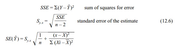
standard error of Yˆ for a given value of x Yˆ ± (t_dfn–2)[SE(Yˆ)] is the confidence interval about Y ˆ ; e.g., t critical is 100(1 – α/2) percentile of Student’s t distribution with n – 2 degrees of freedom.

The sum of squares for error SSE = Σ(Y – Y ˆ )² = 49.56468 (from Table 12.5). The standard error of the estimate refers to the sample standard deviation associated with the deviations about the regression line and is denoted by s_y.x:

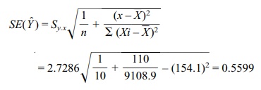
The value S_y.x becomes useful for computing a confidence interval about a predicted value of Y. Previously, we determined that the regression equation for predicting height from weight was height = 59.5944 + 0.0221 weight. For a weight of 110 pounds we predicted a height of 62.02 inches. We would like to be able to compute a confidence interval for this estimate. First we calculate the standard error of the expected Y for a given value of [SE(Y ˆ)]:

The 95% confidence interval is

Y ˆ ± (t_dfn–2)[SE(Yˆ)] 95% CI [62.02 ± 2.306(0.5599)] = [63.31 ↔ 60.73]

We would also like to be able to determine whether the population slope (β) of the regression line is statistically significant. If the slope is statistically significant, there is a linear relationship between X and Y. Conversely, if the slope is not statis-tically significant, we do not have enough evidence to conclude that even a weak linear relationship exists between X and Y. We will test the following null hypothe sis: H_o: β = 0. Let b = estimated population slope for X and Y. The formula for estimating the significance of a slope parameter β is shown in Equation 12.7.

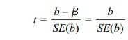
test statistic for the significance of β

(12.7)

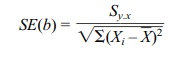
standard error of the slope estimate [SE(b)]

The standard error of the slope estimate [SE(b)] is (note: refer to Table 12.5 and the foregoing sections for the values shown in the formula)

SE(b) = 2.7286/√9108.9 =  0.02859

t = 0.0221/√0.02859  = 0.77

p = n.s.

In agreement with the results for the significance of the correlation coefficient, these results suggest that the relationship between height and weight is not statistically significant These two tests (i.e., for the significance of r and significance of b) are actually mathematically equivalent.

This t statistic also can be used to obtain a confidence interval for the slope, namely [b – t_1–a/2 SE(b), b + t_1–a/2 SE(b)], where the critical value for t is the 100(1 – a/2) percentile for Student’s t distribution with n – 2 degrees of freedom. This interval is a 100(1 – a)% confidence interval for β.

Sometimes we have knowledge to indicate that the intercept is zero. In such cases, it makes sense to restrict the solution to the value a = 0 and arrive at the least squares estimate for b with this added restriction. The formula changes but is easily calculated and there exist computer algorithms to handle the zero intercept case.

When the error terms are assumed to have a normal distribution with a mean of 0 and a common variance σ², the least squares solution also has the property of maximizing the likelihood. The least squares estimates also have the property of being the minmum variance unbiased estimates of the regression parameters [see Draper and Smith (1998) page 137]. This result is called the Gauss–Markov theorem [see Draper and Smith (1998) page 136].