Multiple Regression

MULTIPLE REGRESSION

The only difference between multiple linear regression and simple linear regression is that the former introduces two or more predictor variables into the prediction model, whereas the latter introduces only one. Although we often use a model of Y = a + βX for the form of the regression function that relates the predictor (indepen-dent) variable X to the outcome or response (dependent) variable Y, we could also use a model such as Y = α + βX² or Y = α + β lnX (where ln refers to the log func-tion). The function is linear in the regression parameters α and β.

In addition to the linearity requirement for the regression model, the other re-quirement for regression theory to work is that the observed values of Y differ from the regression function by an independent random quantity, or noise term (error variance term). The noise term has a mean of zero and variance of σ². In addition, σ ² does not depend on X. Under these assumptions the method of least squares pro-vides estimates a and b for α and β, respectively, which have desirable statistical properties (i.e., minimum variance among unbiased estimators).

If the noise term also has a normal distribution, then its maximum likelihood es-timator can be obtained. The resulting estimation is known as the Gauss–Markov theorem, the derivation of which is beyond the scope of the present text. The inter-ested reader can consult Draper and Smith (1998), page 136, and Jaske (1994).

As with simple linear regression, the Gauss–Markov theorem applies to multiple linear regression. For a simple linear regression, we introduced the concept of a noise, or error, term. The prediction equation for multiple linear regression also contains an error term. Let us assume a normally distributed additive error term with variance that is independent of the predictor variables. The least squares esti-mates for the regression coefficients used in the multiple linear regression model exist; under certain conditions, they are unique and are the same as the maximum likelihood estimates [Draper and Smith (1998) page 137].

However, the use of matrix algebra is required to express the least squared esti-mates. In practice, when there are two or more possible variables to include in a re-gression equation, one new issue arises regarding the particular subset of variables that should go into the final regression equation. A second issue concerns the prob-lem of multicollinearity, i.e., the predictor variables are so highly intercorrelated that they produce instability problems.

In addition, one must assess the correlation between the best fitting linear combination of predictor variables and the response variable instead of just a simple cor-relation between the predictor variable and the response variable. The square of the correlation between the set of predictor variables and the response variable is called R², the multiple correlation coefficient. The term R² is interpreted as the percentage of the variance in the response variable that can be explained by the regression function. We will not study multiple regression in any detail but will provide an ex-ample to guide you through calculations and their interpretation.

The term “multicollinearity” refers to a situation in which there is a strong, close to linear relationship among two or more predictor variables. For example, a predic-tor variable X₁ may be approximately equal to 2X₂ + 5X₃ where X₂ and X₃ are two other variables that we think relate to our response variable Y.

To understand the concept of linear combinations, let us assume that we include all three variables (X₁ + X₂ + X₃) in a regression model and that their relationship is exact. Suppose that the response variable Y = 0.3 X₁ + 0.7 X₂ + 2.1 X₃ + ε, where ε is normally distributed with mean 0 and variance 1.

Since X₁ = 2X₂ + 5X₃, we can substitute the right-hand side of this equation into the expression for Y. After substitution we have Y = 0.3(2 X₂ + 5X₃) + 0.7X₂ + 2.1X₃ + ε = 1.3X₂ + 3.6X₃ + ε. So when one of the predictors can be expressed as a linear function of the other, the regression coefficients associated with the predictor vari-ables do not remain the same. We provided examples of two such expressions: Y = 0.3X₁ + 0.7X₂ + 2.1X₃ + ε and Y = 0.0X₁ + 1.3X₂ + 3.6X₃ + ε. There are an infinite number of possible choices for the regression coefficients, depending on the linear combinations of the predictors.

In most practical situations, an exact linear relationship will not exist; even a re-lationship that is close to linear will cause problems. Although there will be (unfor-tunately) a unique least squares solution, it will be unstable. By unstable we mean that very small changes in the observed values of Y and the X’s can produce drastic changes in the regression coefficients. This instability makes the coefficients im-possible to interpret.

There are solutions to the problem that is caused by a close linear relationship among predictors and the outcome variable. The first solution is to select only a subset of the variables, avoiding predictor variables that are highly interrelated (i.e., multicollinear). Stepwise regression is a procedure that can help overcome multi-collinearity, as is ridge regression. The topic of ridge regression is beyond the scope of the present text; the interested reader can consult Draper and Smith (1998), Chapter 17. The problem of multicollinearity is also called “ill-conditioning”; is-sues related to the detection and treatment of regression models that are ill-condi-tioned can be found in Chapter 16 of Draper and Smith (1998). Another approach to multicollinearity involves transforming the set of X’s to a new set of variables that are “orthogonal.” Orthogonality, used in linear algebra, is a technique that will make the X’s uncorrelated; hence, the transformed variables will be well-condi-tioned (stable) variables.

Stepwise regression is one of many techniques commonly found in statistical soft-ware packages for multiple linear regression. The following account illustrates how a typical software package performs a stepwise regression analysis. In stepwise re-gression we start with a subset of the X variables that we are considering for inclusion in a prediction model. At each step we apply a statistical test (often an F test) to de-termine if the model with the new variable included explains a significantly greater percentage of the variation in Y than the previous model that excluded the variable.

If the test is significant, we add the variable to the model and go to the next step of examining other variables to add or drop. At any stage, we may also decide to drop a variable if the model with the variable left out produces nearly the same per-centage of variation explained as the model with the variable entered. The user specifies critical values for F called the “F to enter” and the “F to drop” (or uses the default critical values provided by a software program).

Taking into account the critical values and a list of X variables, the program pro-ceeds to enter and remove variables until none meets the criteria for addition or deletion. A variable that enters the regression equation at one stage may still be re-moved at another stage, because the F test depends on the set of variables currently in the model at a particular iteration.

For example, a variable X may enter the regression equation because it has a great deal of explanatory power relative to the current set under consideration. However, variable X may be strongly related to other variables (e.g., U, V, and Z) that enter later. Once these other variables are added, the variable X could provide little additional explanatory information than that contained in variables U, V, and Z. Hence, X is deleted from the regression equation.

In addition to multicollinearity problems, the inclusion of too many variables in the equation can lead to an equation that fits the data very well but does not do near ly as well as equations with fewer variables when predicting future values of Y based on known values of x. This problem is called overfitting. Stepwise regression is useful because it reduces the number of variables in the regression, helping with overfitting and multicollinearity problems. However, stepwise regression is not an optimal subset selection approach; even if the F to enter criterion is the same as the F to leave criterion, the resulting final set of variables can differ from one another depending on the variables that the user specifies for the starting set.

Two alternative approaches to stepwise regression are forward selection and backward elimination. Forward selection starts with no variables in the equation and adds them one at a time based solely on an F to enter criterion. Backward elim-ination starts with all the variables in the equation and drops variables one at a time based solely on an F to drop criterion. Generally, statisticians consider stepwise re-gression to be better than either forward selection or backward elimination. Step-wise regression is preferred to the other two techniques because it tends to test more subsets of variables and generally settles on a better choice than either forward se-lection or backward elimination. Sometimes, the three approaches will lead to the same subset of variables, but often they will not.

To illustrate multiple regression, we will consider the example of predicting votes for Buchanan in Palm Beach County based on the number of votes for Nader, Gore, and Bush (refer back to Section 12.7). For all counties except Palm Beach, we fit the model Y = α + β₁X₁ + β₂X₂ + β₃X₃ + ε, where X₁ represents votes for Nader, X₂ votes for Bush, and X₃ votes for Gore; ε is a random noise term with mean 0 and variance σ² that is independent of X₁, X₂, and X₃; and α, β₁, β₂, and β₃ are the regression parameters. We will entertain this model and others with one of the predictor variables left out. To do this we will use the SAS procedure REG and will show you the SAS code and output. You will need a statistical computer pack-age to solve most multiple regression problems. Multiple regression, which can be found in most of the common statistical packages, is one of the most widely used applied statistical techniques.

The following three regression models were considered:

1. A model including votes for Nader, Bush, and Gore to predict votes for Buchanan

2. A model using only votes for Nader and Bush to predict votes for Buchanan

3. A model using votes for Nader and Bush and an nteraction term defined as the product of the votes for Nader and the votes for Bush

The coefficient for votes for Gore in model (1) was not statistically significant, so model (2) is probably better than (1) for prediction. Model (3) provided a slightly bet-ter fit than model (2), and under model (3) all the coefficients were statistically sig-nificant. The SAS code (presented in italics) used to obtain the results is as follows:

data florida:

input county $ gore bush buchanan nader;

cards;

alachua 47300 34062 262 3215

baker 2392 5610 73 53

bay 18850 38637 248 828

:

:.

walton 5637 12176 120 265

washngtn 2796 4983 88 93

;

data florid2;

set florida;

if county = ‘palmbch’ then delete;

nbinter = nader*bush;

run;

proc reg;

model buchanan = nader bush gore;

run;

proc reg;

model buchanan = nader bush;

run;

proc reg;

model buchanan = nader bush nbinter;

run;

The data statement at the beginning creates an SAS data set “florida” with “county” as a character variable and “gore bush buchanan and nader” as numeric variables. The input statement identifies the variable names and their formats ($ is the symbol for a character variable). The statement “cards” indicates that the input is to be read from the lines of code that follow in the program.

On each line, a character variable of 8 characters or less (e.g., alachua) first ap-pears; this character variable is followed by four numbers indicating the values for the numeric variables gore, bush, buchanan, and nader, in that order. The process is continued until all 67 lines of counties are read. Note that, for simplicity, we show only the input for the first three lines and the last two lines, indicating with three dots that the other 62 counties fall in between. This simple way to read data is suit-able for small datasets; usually, it is preferable to store data on files and have SAS read the data file.

The next data step creates a modified data set, florid2, for use in the regression modeling. Consequently, we remove Palm Beach County (i.e., the county variable with the value ‘palmbch’). We also want to construct an interaction term for the third model. The interaction between the votes for Nader and the votes for Bush is modeled by the product nader*bush. We call this new variable nbinter.

Now we are ready to run the regressions. Although we could use three model statements in a single regression procedure, instead we performed the regression as three separate procedures. The model statement specifies the dependent variable on the left side of the equation. On the right side of the equation is the list of predictor variables. For the first regression we have the variables nader, bush, and gore; for the second just the variables nader and bush. The third regression specifies nader, bush, and their interaction term nbinter.

The output (presented in bold face) appears as follows:

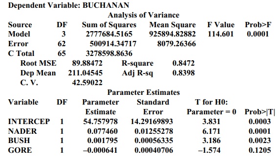
Model: MODEL1 (using votes for Nader, Bush, and Gore to predict votes for Buchanan)

Dependent Variable: BUCHANAN

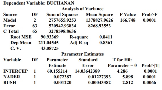
Model: MODEL2 (using votes for Nader and Bush to predict votes for Buchanan)

Dependent Variable: BUCHANAN

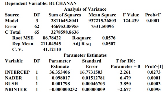
Model: MODEL3 (using votes for Nader and Bush plus an interaction term, Nader*Bush)

Dependent Variable: BUCHANAN

For each model, the value of R² describes the percentage of the variance in the votes for Buchanan that is explained by the predictor variables. By taking into ac-count the joint influence of the significant predictor variables in the model, the adjusted R² provides a better measure of goodness of fit than do the individual predictors. Both models (1) and (2) have very similar R² and adjusted R² values. Model (3) has slightly higher R² and adjusted R² values than does either model (1) or model (2).

The F test for each model shows a p-value less than 0.0001 (the column labeled Prob>F), indicating that at least one of the regression parameters is different from zero. The individual t test on the coefficients suggests the coefficients that are different from zero. However, we must be careful about the interpretation of these results, due to multiple testing of coefficients.

Regarding model (3), since Bush received 152,846 votes and Nader 5564, the equation predicts that Buchanan should have 659.236 votes. Model (1) uses the 268,945 votes for Gore (in addition to those for Nader and Bush) to predict 587.710 votes for Buchanan. Model (2) predicts the vote total for Buchanan to be 649.389. Model (3) is probably the best model, for it predicts that the votes for Buchanan will be less than 660. So again we see that any reasonable model would predict that Buchanan would receive 1000 or fewer votes, far less than the 3407 he actually received!