One-Compartment Open Model: Intravenous Infusion

One-Compartment Open Model

Intravenous Infusion

Rapid i.v. injection is unsuitable when the drug has potential to precipitate toxicity or when maintenance of a stable concentration or amount of drug in the body is desired. In such a situation, the drug (for example, several antibiotics, theophylline, procainamide, etc.) is administered at a constant rate (zero-order) by i.v. infusion. In contrast to the short duration of infusion of an i.v. bolus (few seconds), the duration of constant rate infusion is usually much longer than the half-life of the drug.

Advantages of zero-order infusion of drugs include—

1. Ease of control of rate of infusion to fit individual patient needs.

2. Prevents fluctuating maxima and minima (peak and valley) plasma level, desired especially when the drug has a narrow therapeutic index.

3. Other drugs, electrolytes and nutrients can be conveniently administered simultaneously by the same infusion line in critically ill patients.

The model can be represented as follows:

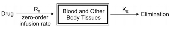
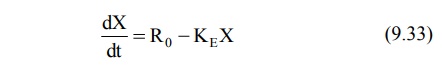
At any time during infusion, the rate of change in the amount of drug in the body, dX/dt is the difference between the zero-order rate of drug infusion R_o and first-order rate of elimination, –K_EX:

Integration and rearrangement of above equation yields:

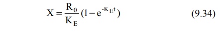
Since X = V_d C, the equation 9.34 can be transformed into concentration terms as follows:

At the start of constant rate infusion, the amount of drug in the body is zero and hence, there is no elimination. As time passes, the amount of drug in the body rises gradually (elimination rate less than the rate of infusion) until a point after which the rate of elimination equals the rate of infusion i.e. the concentration of drug in plasma approaches a constant value called as steady-state, plateau or infusion equilibrium (Fig. 9.3.).

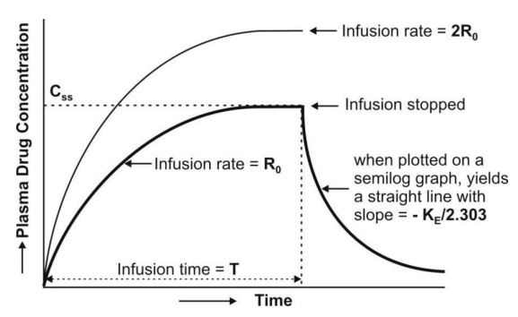
Fig. 9.3. Plasma concentration-time profile for a drug given by constant rate i.v. infusion (the two curves indicate different infusion rates R_o and 2R_o for the same drug)

At steady-state, the rate of change of amount of drug in the body is zero, hence, the equation 9.33 becomes:

Zero = R ₀ - K _E X_ss

or K_E Xss  = R_o (9.36)

Transforming to concentration terms and rearranging the equation:

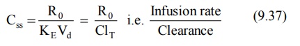
where, X_ss and C_ss are amount of drug in the body and concentration of drug in plasma at steady-state respectively. The value of K_E (and hence t_½) can be obtained from the slope of straight line obtained after a semilogarithmic plot (log C versus t) of the plasma concentration-time data gathered from the time when infusion is stopped (Fig. 9.3). Alternatively, K_E can be calculated from the data collected during infusion to steady-state as follows:

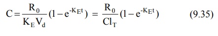
Substituting R_o/Cl_T = C_ss from equation 9.37 in equation 9.35 we get:

C = C ss  _{(1- e}^-KE^t ₎ (9.38)

Rearrangement yields:

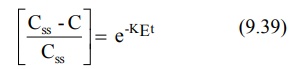
Transforming into log form, the equation becomes:

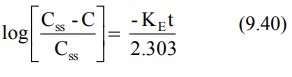
A semilog plot of (C_ss – C)/C_ss versus t results in a straight line with slope –K_E/2.303 (Fig. 9.4).

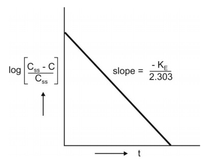
Fig. 9.4 Semilog plot to compute KE from infusion data upto steady-state

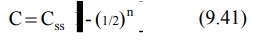
The time to reach steady-state concentration is dependent upon the elimination half-life and not infusion rate. An increase in infusion rate will merely increase the plasma concentration attained at steady-state (Fig. 9.3). If n is the number of half-lives passed since the start of infusion (t/t_½), equation 9.38 can be written as:

The percent of C_ss achieved at the end of each t_½ is the sum of C_ss at previous t_½ and the concentration of drug remaining after a given t_½ (Table 9.3).

TABLE 9.3

Percent of C_ss attained at the end of a given t_½

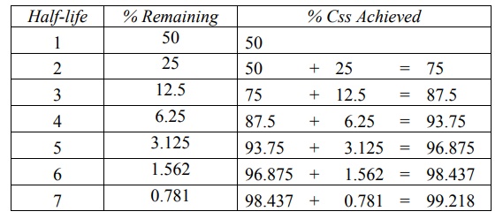
For therapeutic purpose, more than 90% of the steady-state drug concentration in the blood is desired which is reached in 3.3 half-lives. It takes 6.6 half-lives for the concentration to reach 99% of the steady-state. Thus, the shorter the half-life (e.g. penicillin G, 30 min), sooner is the steady-state reached.

Infusion Plus Loading Dose: It takes a very long time for the drugs having longer half-lives before the plateau concentration is reached (e.g. phenobarbital, 5 days). Thus, initially, such drugs have subtherapeutic concentrations. This can be overcome by administering an i.v. loading dose large enough to yield the desired steady-state immediately upon injection prior to starting the infusion. It should then be followed immediately by i.v. infusion at a rate enough to maintain this concentration (Fig. 9.5).

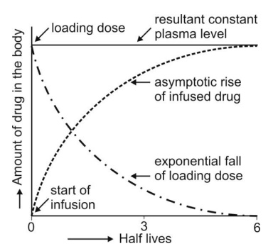
Fig. 9.5 Intravenous infusion with loading dose. As the amount of bolus dose remaining in the body falls, there is a complementary rise resulting from the infusion

Recalling once again the relationship X = V_dC, the equation for computing the loading dose X_o,L can be given:

X_0,LCss V_d           (9.42)

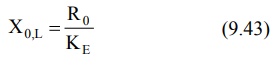
Substitution of C_ss = R_o/K_EV_d from equation 9.37 in above equation yields another expression for loading dose in terms of infusion rate:

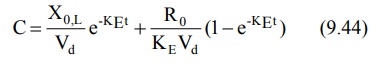
The equation describing the plasma concentration-time profile following simultaneous i.v. loading dose (i.v. bolus) and constant rate i.v. infusion is the sum of two equations describing each process (i.e. modified equation 9.5 and 9.35):

If we substitute C_ssV_d for X_o,L (from equation 9.42) and C_ssK_EV_d for R_o (from equation 9.37) in above equation and simplify it, it reduces to C = C_ss indicating that the concentration of drug in plasma remains constant (steady) throughout the infusion time.

Assessment of Pharmacokinetic Parameters

The first-order elimination rate constant and elimination half-life can be computed from a semilog plot of post-infusion concentration-time data. Equation 9.40 can also be used for the same purpose. Apparent volume of distribution and total systemic clearance can be estimated from steady-state concentration and infusion rate (equation 9.37). These two parameters can also be computed from the total area under the curve (Fig. 9.3) till the end of infusion:

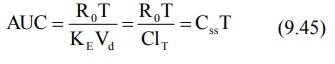
where, T = infusion time.

The above equation is a general expression which can be applied to several pharmacokinetic models.