Two-Compartment Open Model: Intravenous Bolus Administration
| Home | | Biopharmaceutics and Pharmacokinetics |Chapter: Biopharmaceutics and Pharmacokinetics : Compartment Modelling
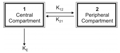
The model can be depicted as shown below with elimination from the central compartment.
Two-Compartment Open Model
Intravenous Bolus Administration
The model can be depicted as shown below with
elimination from the central compartment.
After the i.v. bolus of a drug that follows
two-compartment kinetics, the decline in plasma concentration is biexponential
indicating the presence of two
disposition processes viz. distribution
and elimination. These two processes are not evident to the eyes in a
regular arithmetic plot but when a
semilog plot of C versus t is made, they can be identified (Fig. 9.12).
Initially, the concentration of drug in the central compartment declines rapidly; this is due to the
distribution of drug from the central compartment to the peripheral
compartment. The phase during which this occurs is therefore called as the distributive phase. After sometime, a pseudo-distribution equilibrium is
achieved between the two compartments following which the subsequent loss of
drug from the central compartment is slow and mainly due to elimination. This second, slower rate process is called as the
post-distributive or elimination phase. In contrast to the
central compartment, the drug concentration
in the peripheral compartment first increases and reaches a maximum. This
corresponds with the distribution phase. Following peak, the drug concentration
declines which corresponds to the post-distributive phase (Fig.9.12).

Fig. 9.12. Changes in drug concentration in
the central (plasma) and the peripheral compartment
after i.v. bolus of a drug that fits two-compartment model.
Let K12 and K21 be the
first-order distribution rate constants depicting drug transfer between the
central and the peripheral compartments and let subscript c and p define
central and peripheral compartment respectively. The rate of change in drug
concentration in the central compartment is given by:
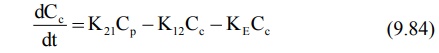
Extending the relationship X = VdC to
the above equation, we have
where Xc and Xp are the
amounts of drug in the central and peripheral compartments respectively and Vc
and Vp are the apparent volumes of the central and the peripheral compartment
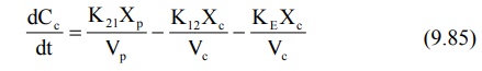
respectively. The rate of change in drug concentration in the peripheral
compartment is given by:
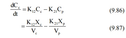
Integration of equations 9.85 and 9.87 yields
equations that describe the concentration of drug in the central and peripheral
compartments at any given time t:
where Xo = i.v. bolus dose, α and β are hybrid first-order constants
for the rapid distribution phase and the slow elimination phase respectively
which depend entirely upon the first-order constants K12, K21
and KE.
The constants K12 and K21 that depict reversible transfer of drug between compartments are
called as microconstants or
transfer constants. The
mathematical relationships between
hybrid and microconstants are given as:
α + β = K12 + K21 + KE (9.90)
αβ = K21KE (9.91)
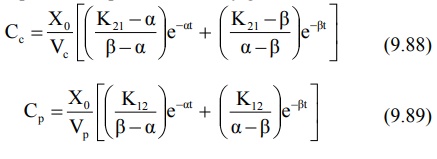
Equation 9.88 can be written in simplified form as:
Cc = Ae –αα + Be βt (9.92)
Cc = Distribution exponent Elimination
exponent
where A and B are also hybrid constants for the two
exponents and can be resolved graphically by the method of residuals.
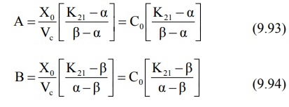
where Co = plasma drug concentration
immediately after i.v. injection.
Method of Residuals: The
biexponential disposition curve obtained after i.v. bolus of a drug that fits two compartment model
can be resolved into its individual exponents by the method of residuals.
Rewriting the equation 9.92:
Cc = Ae -αα + Be -βt (9.92)
As apparent from the biexponential curve given in
Fig. 9.12., the initial decline due to distribution is more rapid than the
terminal decline due to elimination i.e. the rate constant α >> ß and hence the term e–αt approaches zero much faster than does e–βt. Thus, equation 9.92 reduces to:
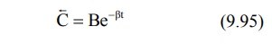
In log form, the equation
where C = back extrapolated plasma concentration
values. A semilog plot of C versus t yields the terminal linear phase of the
curve having slope –β/2.303 and when back extrapolated
to time zero, yields y-intercept log B (Fig. 9.13.).The t½ for the
elimination phase can be obtained from equation t½ = 0.693/β.
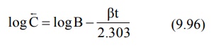
Subtraction of extrapolated plasma concentration
values of the elimination phase (equation 9.95) from the corresponding true
plasma concentration values (equation 9.92) yields a series of residual
concentration values Cr.
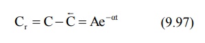
In log form, the equation becomes:
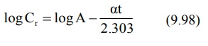
A semilog plot of Cr versus t yields a straight line with slope –α/2.303 and Y-intercept log A (Fig. 9.13).
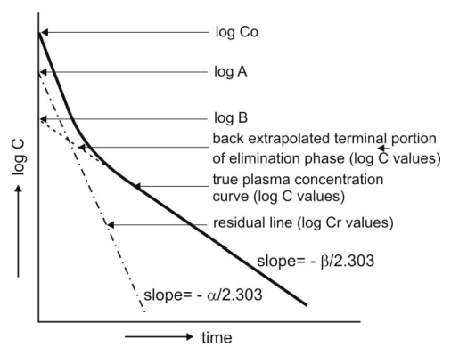
Fig. 9.13. Resolution of biexponential
plasma concentration-time curve by the method of residuals for a drug that follows two-compartment kinetics on i.v.
bolus administration.
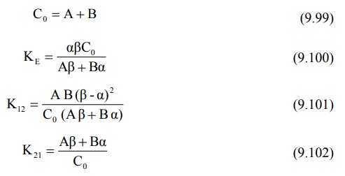
Assessment of Pharmacokinetic Parameters: All the parameters of equation 9.92 can be resolved by the method of residuals as described above. Other
parameters of the model viz. K12, K21, KE,
etc. can now be derived by proper substitution of these values.
C0 = A + B (9.99)
It must be noted that for two-compartment model, KE
is the rate constant for elimination of drug from the central compartment and β is the rate constant for
elimination from the entire body.
Overall elimination t½ should
therefore be calculated from β.
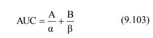
Area under the plasma concentration-time curve can
be obtained by the following equation:
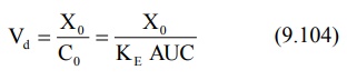
The apparent volume of central compartment Vc
is given as:
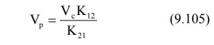
Apparent volume of peripheral compartment can be
obtained from equation:
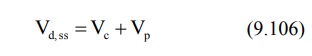
The apparent volume of distribution at steady-state
or equilibrium can now be defined as:
It is also given as:
Total systemic clearance is given as:
The pharmacokinetic parameters can also be
calculated by using urinary excretion data:
An equation identical to equation 9.92 can be
derived for rate of excretion of unchanged drug in urine:
The above equation can be resolved into individual
exponents by the method of residuals as described for plasma concentration-time
data.
Renal clearance is given as:
ClR Ke Vc (9.111)
Related Topics
