Michaelis Menten Equation

MICHAELIS MENTEN EQUATION

The kinetics of capacity-limited or saturable processes is best described by Michaelis-

Menten equation:

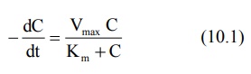
Where,

–dC/dt = rate of decline of drug concentration with time,

V_max = theoretical maximum rate of the process, and

K_m = Michaelis constant.

Three situations can now be considered depending upon the values of K_m and C:

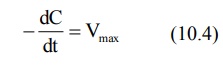
1. When K_m = C

Under this situation, the equation 10.1 reduces to:

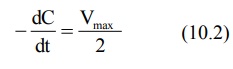
i.e. the rate of process is equal to one-half its maximum rate (Fig. 10.1).

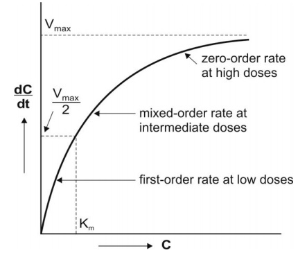
Fig. 10.1 A plot of Michaelis-Menten equation (elimination rate dC/dt versus concentration C). Initially, the rate increases linearly (first-order) with concentration, becomes mixed-order at higher concentration and then reaches maximum (Vmax) beyond which it proceeds at a constant rate (zero-order).

2. When K_m >> C

Here, K_m + C ≡ K_m and the equation 10.1 reduces to:

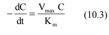
The above equation is identical to the one that describes first-order elimination of a drug where V_max/K_m = K_E. This means that the drug concentration in the body that results from usual dosage regimens of most drugs is well below the K_m of the elimination process with certain exceptions such as phenytoin and alcohol.

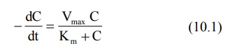
3. When K_m << C

Under this condition, K_m + C ≡ C and the equation 10.1 will become:

The above equation is identical to the one that describes a zero-order process i.e. the rate process occurs at a constant rate V_max and is independent of drug concentration e.g. metabolism of ethanol.

Estimation of K_m and V_max

The parameters of capacity-limited processes like metabolism, renal tubular secretion and biliary excretion can be easily defined by assuming one-compartment kinetics for the drug and that elimination involves only a single capacity-limited process.

The parameters K_m and V_max can be assessed from the plasma concentration-time data collected after i.v. bolus administration of a drug with nonlinear elimination characteristics.

Rewriting equation 10.1.

Integration of above equation followed by conversion to log base 10 yields:

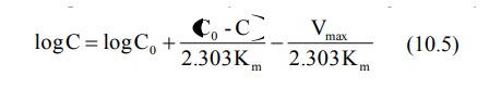
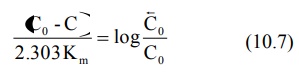
A semilog plot of C versus t yields a curve with a terminal linear portion having slope –V_max/2.303K_m and when back extrapolated to time zero gives Y-intercept log BarC₀ () (see Fig. 10.2). The equation that describes this line is:

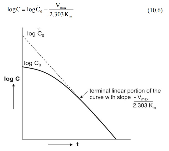
Fig. 10.2 Semilog plot of a drug given as i.v. bolus with nonlinear elimination and that fits one-compartment kinetics.

At low plasma concentrations, equations 10.5 and 10.6 are identical. Equating the two and simplifying further, we get:

K_m can thus be obtained from above equation. V_max can be computed by substituting the value of K_m in the slope value.

An alternative approach of estimating V_max and K_m is determining the rate of change of plasma drug concentration at different times and using the reciprocal of the equation 10.1. Thus:

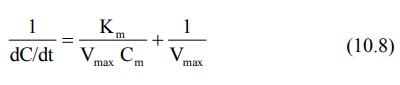
where C_m = plasma concentration at midpoint of the sampling interval. A double reciprocal plot or the Lineweaver-Burke plot of 1/(dC/dt) versus 1/C_m of the above equation yields a straight line with slope = K_m/V_max and y-intercept = 1/V_max.

A disadvantage of Lineweaver-Burke plot is that the points are clustered. More reliable plots in which the points are uniformly scattered are Hanes-Woolf plot (equation 10.9) and Woolf-Augustinsson-Hofstee plot (equation 10.10).

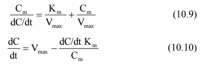
The above equations are rearrangements of equation 10.8. Equation 10.9 is used to plot C_m/(dC/dt) versus C_m and equation 10.10 to plot dC/dt versus (dC/dt)/C _m. The parameters K_m and V_max can be computed from the slopes and y-intercepts of the two plots.

K_m and V_max from Steady-State Concentration

When a drug is administered as a constant rate i.v. infusion or in a multiple dose regimen, the steady-state concentration C_ss is given in terms of dosing rate DR as:

DR = C_ssCl_T                            (10.11)

where DR = R_o when the drug is administered as zero-order i.v. infusion and it is equal to FX_o/τ when administered as multiple oral dosage regimen (F is fraction bioavailable, X_o is oral dose and is dosing interval).

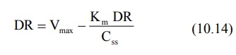
At steady-state, the dosing rate equals rate of decline in plasma drug concentration and if the decline (elimination) is due to a single capacity-limited process (for e.g. metabolism), then;

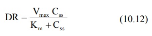
A plot of C_ss versus DR yields a typical hockey-stick shaped curve as shown in Fig. 10.3.

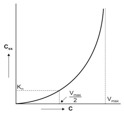
Fig. 10.3 Curve for a drug with nonlinear kinetics obtained by plotting the steady-state concentration versus dosing rates.

To define the characteristics of the curve with a reasonable degree of accuracy, several measurements must be made at steady-state during dosage with different doses.

Practically, one can graphically compute Km and Vmax in 3 ways:

1. Lineweaver-Burke Plot/Klotz Plot

Taking reciprocal of equation 10.12, we get:

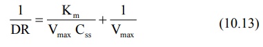
Equation 10.13 is identical to equation 10.8 given earlier. A plot of 1/DR versus 1/C_ss yields a straight line with slope K_m/V_max and y-intercept 1/V_max (see Fig. 10.4).

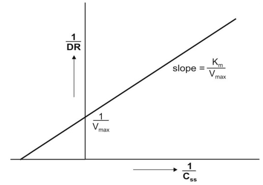
Fig. 10.4 Lineweaver-Burke/Klotz plot for estimation of Km and Vmax at steady-state concentration of drug.

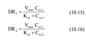
2. Direct Linear Plot

Here, the graph is considered as shown in Fig. 10.5. A pair of C_ss viz. C_ss,1 and C_ss,2 obtained with two different dosing rates DR₁ and DR₂ is plotted. The points C_ss,1 and DR₁ are joined to form a line and a second line is obtained similarly by joining C_ss,2 and DR₂. The point where these two lines intersect each other is extrapolated on DR axis to obtain V_max and on x-axis to get K_m.

Fig. 10.5 Direct linear plot for estimation of K_m and V_max at steady-state concentrations of a drug given at different dosing rates.

3. The third graphical method of estimating K_m and V_max involves rearranging equation 10.12 to yield:

A plot of DR versus DR/C_ss yields a straight line with slope -K_m and Y-intercept V_max^.

K_m and V_max can also be calculated numerically by setting up simultaneous equations as shown below:

Combination of the above two equations yields:

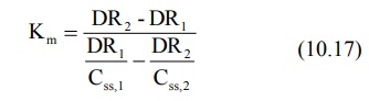
After having computed K_m, its subsequent substitution in any one of the two simultaneous equations will yield V_max.

It has been observed that K_m is much less variable than V_max. Hence, if mean K_m for a drug is known from an earlier study, then instead of two, a single measurement of C_ss at any given dosing rate is sufficient to compute V_max.

There are several limitations of K_m and V_max estimated by assuming one-compartment system and a single capacity-limited process. More complex equations will result and the computed K_m and V_max will usually be larger when:

1. The drug is eliminated by more than one capacity-limited process.

2. The drug exhibits parallel capacity-limited and first-order elimination processes.

3. The drug follows multicompartment kinetics.

However, K_m and V_max obtained under such circumstances have little practical applications in dosage calculations. 

Drugs that behave nonlinearly within the therapeutic range (for example, phenytoin shows saturable metabolism) yield less predictable results in drug therapy and possess greater potential in precipitating toxic effects.