Statistical measures

Statistical measures

A pharmacist needs to be aware of how the scientific data are generated and interpreted in the modern evidence-based medicine. This is important not only for the adequate appreciation and interpretation of new research findings but also for an understanding of conventionally well-established practices in medicine. This section outlines the basic concepts utilized in the generation and interpretation of data. It assumes the background knowl-edge of experimental design and random sampling.

Measures of central tendency

When a collection of data is available, it can be arranged in an array. An array is a collection of data arranged in a systematic manner, such as listing a set of values in an ascending or descending order of their mag-nitude. The data can be analyzed in terms of their frequency distribution. The frequency distribution is constructed by identifying the number of times a value repeats itself (frequency of occurrence of such value). This information can be plotted in a two-dimensional x–y plot, with the x-axis representing the increasing order of values and the y-axis representing their frequency of occurrence. The frequency distribution can also be organized to represent a set of ranges of values, rather than individual values, with the frequency representing all data points that fall within the given ranges. An x–y plot of this range of values can produce a series of columns, called a histogram. These approaches both reduce and organize the data for easy interpretation.

Frequently, when the data are organized in a frequency distribution, a normal distribution is obtained (Figure 5.4).

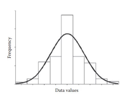
Figure 5.4 A normal distribution. Normal distribution of data can be represented by (a) frequency distribution (histogram), (b) a curve passing through the medians of the frequency distribution, and (c) discrete data points.

A review of the normal distribution curve indicates that the data tend to be more frequent for a given set of values, which are usually toward the center of the numerical distribution of data values. This is called central tendency. The numeric location of the central tendency can be stated in one of three ways: mean, median, and mode.

·           Mean: The arithmetic mean of a data is the sum of observations divided by the number of observations. The mean describes the central location of the data.

·           Median: The median is the numeric value of a data point that falls in the middle when counting the set of values after arranging them in an ascending or descending order.

·           Mode: Mode is the value that occurs most frequently in a set of data.

Either of these values tends to indicate the numeric point in the spread of the data that all observations tend to lean toward, which can be interpreted as the expected value of a data set. The expected value of a distribution is the average, or the first moment, over the entire distribution. Each and every value in the data set is not the expected value due to random variation or errors in experimentation or data collection.

Measures of dispersion

In addition to knowing the central tendency of the data, one needs to appre-ciate the level of distribution or variation in the individual data values. This indicates how closely the data set represents a central tendency or value. For example, the four sets of data represented by the normal distribution curves in Figure 5.5 show increasing level of dispersion from the central tendency in the order a < b < c < d.

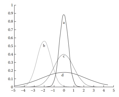
Figure 5.5 Illustration of variability in four different data sets following normal distribution. The level of dispersion from the central tendency is d > c > a, even though their means are the same. Data set b represents a difference of mean in addition to dispersion.

Distribution of a set of data can be quantified by one or more of the following numerical values:

·           Range: It represents the difference between the highest and the lowest values in a data set.

·           Variance and standard deviation: Variance represents the mean of square of deviation of all individual values in the data set from the mean of the set of data set. It is calculated by subtracting each indi-vidual value from the mean, squaring it, and dividing the sum of this squared difference by n−1, where n is the number of samples in the data set. Standard deviation is the square root of the variance.

Standard deviation is commonly used to interpret the spread of the data. As indicated in Figure 5.6, assuming a normal sample distribution, the stan-dard deviation of a sample set (symbol: s) indicates the percentage of data set values that fall on either side of the mean value of this data set. As illus-trated in the figure, 68.26% of values fall within ±1 s of the mean, 95.44% fall within ±2 s of the mean, and 99.72% fall within ±3 s of the mean. It would be noted that the greater the value of s compared with the mean, the more the spread of the data. This could indicate either lower precision of measurement and/or greater error in data collection.

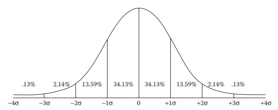
Figure 5.6 Illustration of spread of data (from the hypothetical mean of 0) in a normal distribution as a function of the standard deviation of the population (σ). The probability of finding data values at illustrated multiples of standard deviation is indicated in the figure as a percentage number.

Sample probability distributions

A probability distribution represents the probability of occurrence of each value of a discrete random variable or the probability of each value of a continuous random variable falling within a given interval. Hence, a probability distribution can be either:

·           Discrete probability distribution: It reflects a finite and countable set of data whose probability is one.

·           Continuous probability distribution: It reflects the probability of occurrence of a value in terms of its probability density function, which can be defined within an interval.

1. Normal distribution

The preceding examples assumed a normal frequency or probability dis-tribution of the data set. Normal distribution, also known as the Gaussian distribution, reflects the tendency of the data to cluster around the mean from both directions. It is a continuous probability distribution and forms a typical bell-shaped curve. A data set following a normal distribution is indicative of the additive nature of underlying factors.

2. Log-normal distribution

A log-normal distribution refers to the probability distribution of a variable whose logarithm is normally distributed, such that for a variable y, log y is normally distributed. The base of the logarithmic function does not make a difference to the distribution pattern of the variable. A log-normal distribu-tion typically represents a multiplicative effect of underlying factors.

3. Binomial distribution

Binomial distribution is a discrete probability distribution that reflects the number of a given outcome in a sequence of experiments with only two outcomes, each of which yields a given outcome with a defined probability. Such an experiment is frequently called a success/failure experiment or Bernoulli experiment, with n repetitions and p as the probability of each successful outcome.

4. Poisson distribution

Poisson distribution represents the probability of n occurrences of an event over a period of time or space, given the average number of occurrences of the event. For example, if the lyophilization process fails, on an average, in five batches per year, the Poisson distribution can be used to calculate the probability of 0, 1, 2, 3, 4, 5, … failed lyophilization processes for a given year. Although both Poisson and binomial distributions are based on dis-crete random variables, the binomial distribution assumes a finite number of possible outcomes, while the Poisson distribution does not. The Poisson distribution is usually applied in cases where the mean is much smaller than the maximum data value possible, such as in radioactive decay.

5. Student’s t-distribution

The Student’s t-distribution is a continuous probability distribution that is used to estimate the mean of a normally distributed population when the sample size is small (population standard deviation is unknown). The t-distribution is based on the central limit theorem that the sampling distribution of a sample statistic, such as the sample mean (x), follows a normal distribution as n gets large. The t-distribution is a continuous probability distribution of the t-statistic or t-score, defined as:

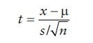
where:

μ is the population mean

s is the sample standard deviation

n is the sample size

The shape of the t-distribution varies with the sample size or the number of degrees of freedom (df) of the sample. The degrees of freedom represent the number of values in the final calculation of a statistic that can freely vary and is calculated as n−1 for n number of samples. It is used as a measure of the amount of data that is used for the estimation of a given statistical parameter.

The t-distribution is characterized by having a mean of 0 and variance of always greater than 1. The variance approaches 1, and the t-distribution approaches the standard normal distribution at high sample sizes.

Knowing the sample mean, standard deviation, size, and the (assumed) population mean, a t-score or t-statistic can be calculated. Each t-score is associated with a unique cumulative probability of finding a sample mean less than or equal to the chosen sample mean for a random sample of the same size. The term t_α denotes a t-score that has a cumulative probability of (1α). For example, for a cumulative probability of occurrence of 95%, α= (1–95/100) = 0.05. Hence, the t-score corresponding to this probability would be represented as t_0.05. The t-score for a given probability varies with the degrees of freedom (DF) of the sample. Thus, t_0.05 at DF of 2 is 2.92, whereas t_0.05 at DF of 20 is 1.725. In addition, since t-distribution is symmetric with a mean of zero, t_0.05 = −t_0.95, or vice versa.

The t-statistic helps determine the probability of occurrence of a given sample mean when the (hypothetical or target) population mean is known. In other words, it can help determine the probability that the selected sample comes from the population with the given (hypothetical or target) mean. For example, during tablet compression for a target average tablet weight of 100 mg, a sample of 10 tablets is weighed. The average weight of 10 tablets was 90 mg, with a standard deviation of 35 mg. What is the probability that the tablet compression operation is proceeding at its target average tablet weight of 100 mg? To compute this probability, a t-score can be calculated as follows:

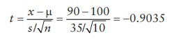
This t-score corresponds to 19% probability of occurrence (using standard probability distribution tables). Thus, if the tableting operation is performing at target, then there is a 19% chance that the sample mean would fall below 90, based on a sample of 10 tablets. Therefore, there is no evidence that the machine is off target. However, due to the large variability and small sample size, we cannot say that it is at target. A confidence interval would show that the target mean could be any value over a large range, which would include 100. Thus, it is likely that the tableting unit operation is per-forming at the target average tablet weight of 100 mg. On the other hand, if the sample of 10 tablets had a standard deviation of 15 mg, the t-score would be 2.1082, which corresponds to the probability of occurrence of 3%. These data would indicate that the tableting unit operation is probably not performing at its target average tablet weight of 100 mg.

This distribution forms the basis of the t-test of significance, which can help determine the following:

·           Statistical significance of the difference between two sample means.

·           Confidence intervals for the difference between two population means.

6. Chi-square distribution

Chi-square (χ²) distribution represents the squared ratio of sample to population standard deviation as a function of the sample size used for computing the sample standard deviation. This distribution is used to estimate the probability ranges for the standard deviation values for a given sample size.

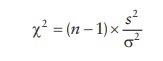
Mathematically, the chi-square distribution represents the distribution of the chi-square statistic, which represents the squared ratio of the standard deviation of a sample (s) to that of the population (σ), multiplied by the degrees of freedom of the sample.

The shape of the chi-square distribution curve varies as a function of the sample size or the degrees of freedom. As the number of degrees of freedom increases, the chi-square curve approaches a normal distribution.

The chi-square distribution is constructed such that the total area under the curve is 1. This allows the estimation of cumulative probability of a given value of the chi-square parameter. Given this value, the probability of occurrence of the chi-square parameter above the obtained value can be obtained.

For example, for a population of N = 100 with the population standard deviation of 5, the probability of obtaining a sample standard deviation of 6 when testing n = 10 samples is given by the chi-square parameter,

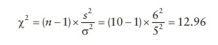
Using the chi-square distribution for the given degrees of freedom, the probability of occurrence of chi-square parameter less than 12.96 is 0.84. Hence, the probability of occurrence of s > 6 is 1 – 0.84 = 0.16, or 16%.