Diffusion rate
| Home | | Pharmaceutical Drugs and Dosage | | Pharmaceutical Industrial Management |Chapter: Pharmaceutical Drugs and Dosage: Biopharmaceutical considerations
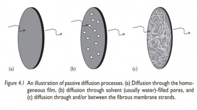
Fick’s first law of diffusion describes the diffusion process under steady state when the concentration gradient (dC/dx) does not change with time. The second law refers to a change in the concentration of diffusant with time at any distance.
Diffusion rate
Fick’s
first law of diffusion describes the diffusion process under steady state when
the concentration gradient (dC/dx) does not change with time. The second
law refers to a change in the concentration of diffusant with time at any
distance (i.e., a nonsteady state). Diffusive transport from a dosage form is
usually slow, leading to most of the drug transport happen-ing under
steady-state conditions. Therefore, it is important to understand the diffusive
conditions under a steady state.
Diffusion cell
Figure 4.2 shows the schematic of a diffusion cell, with a diaphragm of thickness
h and cross-sectional area S separating the two compartments. A
concentrated solution of drug is loaded in the donor compartment and allowed to
diffuse into the solvent in the receptor compartment. The solvent in both the
compartments is continuously mixed and sampled frequently to quantitate drug
transport across the membrane.
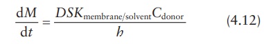
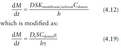
Equating
both equations for flux, Fick’s first law of diffusion may be written as:
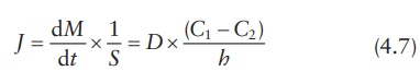
in
which (C1 − C2)/h approximates dC /dx. Concentrations C1 and C2 within the membrane (Figure
4.2) are determined by the partition coefficient of the solute (Kmembrane/solvent) multiplied
by the concentration in the donor com-partment (Cdonor) or in the receptor compartment (Creceptor). Thus, we have:
C1 = Cdonor × Kmembrane solvent (4.8)
and
C2 = Creceptor × Kmembrane solvent (4.9)
Therefore,
the partition coefficient is given by:
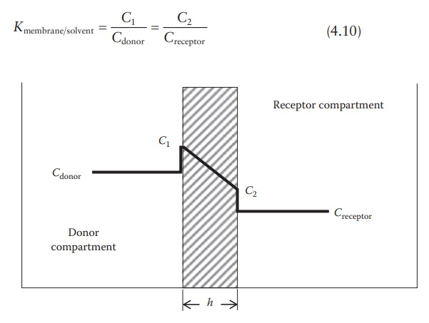
Figure 4.2 Drug concentrations in a
diffusion cell.
Hence,
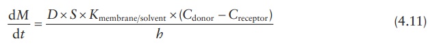
Under sink conditions, the drug concentration in the receptor compart-ment is maintained much lower than the drug concentration in the donor compartment, such that Creceptor → 0. Therefore, the above equation can be simplified as:
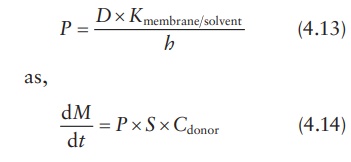
This
equation can also be expressed in terms of the permeability coeffi-cient, P, in cm/s, which is defined as:
Spherical membrane-controlled drug delivery system
Following
the same principles as outlined above for a diffusion cell, dif-fusive drug
release from a spherical rate-limiting membrane enclosing a drug solution can
be defined in terms of the surface area of the membrane at the center point of
its thickness and the linear distance of drug diffusion across the membrane, x. Given the inner-boundary radius of
the membrane as rinner and
the outer-boundary radius of the membrane as router, the surface area of the sphere at its mean
radius is given by:
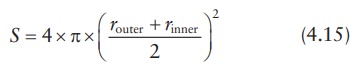
The
surface area of the sphere may be approximated by:
S = 4 × π × router × rinner (4.16)
And
the linear distance for solute diffusion across the membrane is given by:
x = router – rinner (4.17)
Thus,
the expression for the drug-release rate from a sphere is:
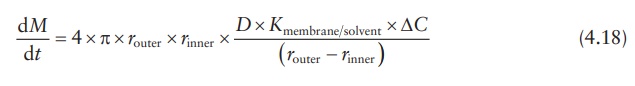
where
ΔC is the concentration gradient
between the inside and the outside of the membrane.
Thus,
permeability depends on both the properties of the diffusing solute (partition
coefficient and diffusion coefficient) and the properties of the membrane
(thickness and surface area).
Pore diffusion
In
microporous reservoir systems, drug molecules are released by diffusion through
the solvent-filled micropores. Drug transport across such porous membranes is
termed pore diffusion. In this system, the pathway of drug transport is no
longer straight but tortuous. The rate of drug transport is directly
proportional to the porosity, ε,
of the membrane and inversely pro-portional to the tortuosity, τ, of the pores. In addition, the
partition coef-ficient of the drug between the membrane and the solvent (Kmembrane solvent) is no
longer a factor, since drug dissolution in the membrane is not required.
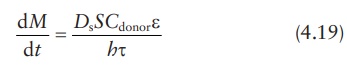
Therefore,
In
this modified equation, Ds
is the drug diffusion coefficient in the solvent.
Determining permeability coefficient
Using
the permeability coefficient:
where,
surface area is given by:
S = 4 × π × router × rinner (4.16)
and
concentration gradient is given by ΔC = Cdonor − Creceptor, with the assumption
that Creceptor → 0 under sink conditions; thus, if ΔC ≅ Cdonor , we obtain:
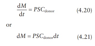
Thus, the value of permeability coefficient, P, can be obtained from the slope of a linear plot of M versus t, provided that Cdonor remains relatively constant.
Lag time in non-steady state diffusion
sustained-release
dosage form may not exhibit a steady-state phenom-enon from the initial time of
drug release. For example, the rate of drug diffusion across a membrane slowly
increases to steady-state kinetics (Figure 4.3).
As shown in this figure, the curve is convex to the time axis in the early
stage and then becomes linear. This early stage is the nonsteady-state
condition. Later, the rate of diffusion is constant, the curve is essen-tially
linear, and the system is at a steady state. When the steady state portion of
the line is extrapolated to the time axis, the point of intersection represents
the time of zero diffusion concentration if the system had been at the steady
state all along. This time period between the actual nonsteady state and the
projected steady-state time at zero diffusion concentration is known as the lag
time. This is the time required for a penetrant to establish a uniform
concentration gradient within the membrane that separates the donor from the
receptor compartments.
Matrix (monolithic)-type non-degradable system
In
a matrix-type polymeric delivery system, the drug is distributed through-out a
polymeric matrix. The drug may be dissolved or suspended in the polymer.
Regardless of a drug’s physical state in the polymeric matrix, the
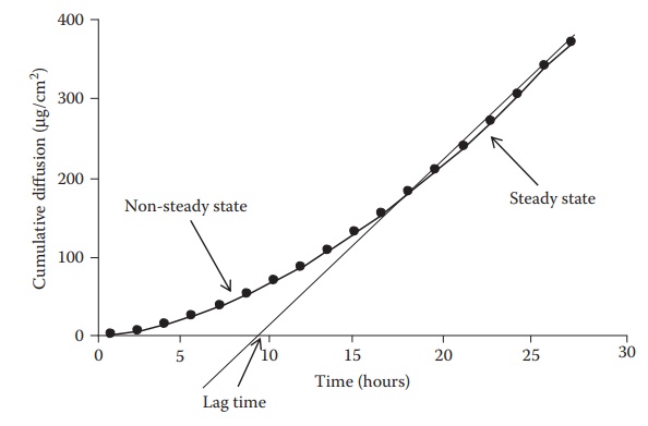
Figure 4.3 Drug diffusion rate across a
polymeric membrane.
In these systems, drug molecules can elute out
of the matrix only by dissolution in the surrounding poly-mer (if drug is
suspended) and by diffusion through the polymer structure. Initially, drug
molecules closest to the surface are released from the device. As drug release
continues, molecules must travel a greater distance to reach the exterior of
the device. This increases the diffusion time required for drug-release. This
increase in diffusion time results in a decrease in the drug-release rate from
the device with time.
In
an insoluble matrix-type system, the drug-release rate decreases over time as a
function of the square root of time (Higuchi, 1963).
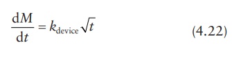
where
kdevice is a
proportionality constant dependent on the properties of the device.
This
release kinetics is observed for the release of the first 50%–60% of the total
drug content. Thereafter, the release rate usually declines expo-nentially.
Thus, the reservoir system can provide constant release with time (zero-order
release kinetics), whereas a matrix system provides decreasing release with
time (square root of time-release kinetics).
Calculation examples
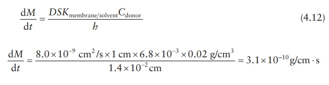
Drug-release rate
Calculation
of diffusion coefficient across and partition coefficient into a membrane
barrier of a drug delivery system is often undertaken to simulate drug-release
rate kinetics under different formulation conditions, such as drug loading. The
diffusion rate may be calculated by using experimental data in one set of
experiments. For example, if it were known that the diffusion coefficient of
tetracycline in a hydroxyethyl methacrylate–methyl methacrylate copolymer film
is D = 8.0(±4.7) × 10–9 cm2/s
and the partition coefficient, K, for
tetracycline between the membrane and the reservoir fluid of the drug delivery
device is 6.8(±5.9) × 10–3, drug-release rate can be calculated if
the design parameters of the device are known. If the mem-brane thickness, h,
of the device is 1.4 × 10⁻² cm and the concentration of tetracycline
in the core, Ccore, is
0.02 g/cm3, tetracycline-release rate, dM/dt, may be calculated
as follows.
To obtain the results in micrograms per day,
dM / dt = 3 . 1× 10⁻¹⁰ g/cm ⋅ s × 106 µg/g × 60 × 60 × 24 s/day = 26.85 µg/day ⋅
cm
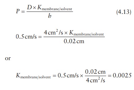
Partition coefficient
Knowing
the permeability coefficient and the diffusion coefficient of a drug in a
membrane, its partition coefficient can be calculated. For example, if a new
glaucoma drug diffuses across a barrier of 0.02 cm with a permeability
coefficient of 0.5 cm/s and the diffusion coefficient is 4 cm2/s,
its perme-ability coefficient may be calculated as follows:
Related Topics