Sensitivity to Outliers, Outlier Rejection, and Robust Regression

SENSITIVITY TO OUTLIERS, OUTLIER REJECTION, AND ROBUST REGRESSION

Outliers refer to unusual or extreme values within a data set. We might expect many biochemical parameters and human characteristics to be normally distributed, with the majority of cases falling between ±2 standard deviations. Nevertheless, in a large data set, it is possible for extreme values to occur. These extreme values may be caused by actual rare events or by measurement, coding, or data entry errors. We can visualize outliers in a scatter diagram, as shown in Figure 12.4.

The least squares method of regression calculates “b” (the regression slope) and  “a” (the intercept) by minimizing the sum of squares [Σ(Y – Yˆ)²] about the regression line. Outliers cause distortions in the estimates obtained by the least squares method. Robust regression techniques are used to detect outliers and minimize their influence in regression analyses.

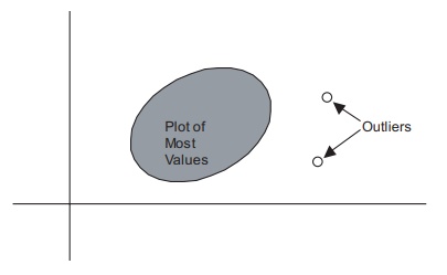
Figure 12.4. Scatter diagram with outliers.

Even a few outliers may impact both the intercept and the slope of a regression line. This strong impact of outliers comes about because the penalty for a deviation from the line of best fit is the square of the residual. Consequently, the slope and in-tercept need to be placed so as to give smaller deviations to these outliers than to many of the more “normal” observations.

The influence of outliers also depends on their location in the space defined by the distribution of measurements for X (the independent variable). Observations for very low or very high values of X are called leverage points and have large effects on the slope of the line (even when they are not outliers). An alternative to least squares regression is robust regression, which is less sensitive to outliers than is the least squares model. An example of robust regression is median regression, a type of quantile regression, which is also called a minimum absolute deviation model.

A very dramatic example of a major outlier was the count of votes for Patrick Buchanan in Florida’s Palm Beach County in the now famous 2000 presidential election. Many people believe that Buchanan garnered a large share of the votes that were intended for Gore. This result could have happened because of the confus-ing nature of the so-called butterfly ballot.

In any case, an inspection of two scatter plots (one for vote totals by county for Buchanan versus Bush, Figure 12.5, and one for vote totals by county for Buchanan versus Gore, Figure 12.6) reveals a consistent pattern that enables one to predict the number of votes for Buchanan based on the number of votes for Bush or Gore. This prediction model would work well in every county except Palm Beach, where the votes for Buchanan greatly exceeded expectations. Palm Beach was a very obvious outlier. Let us look at the available data published over the Internet.

Table 12.6 shows the counties and the number of votes that Bush, Gore, and Buchanan received in each county. The number of votes varied largely by the size of the county; however, from a scatter plot you can see a reasonable linear relationship between; for instance, the total number of votes for Bush and the total number for Buchanan. 

TABLE 12.6. 2000 Presidential Vote by County in Florida

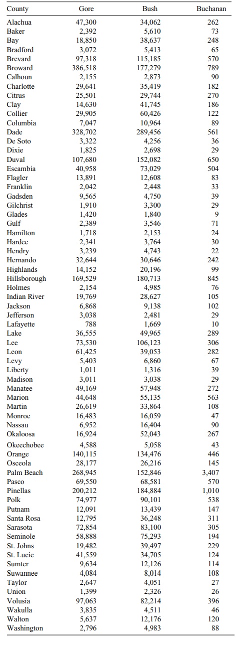
One could form a regression equation to predict the total number of votes for Buchanan given that the total number of votes for Bush is known. Palm Beach County stands out as a major exception to the pattern. In this case, we have an outlier that is very informative about the problem of the butterfly ballots.

Palm Beach County had by far the largest number of votes for Buchanan (3407 votes). The county that had the next largest number of votes was Pinellas County, with only 1010 votes for Buchanan. Although Palm Beach is a large county, Broward and Dade are larger; yet, Buchanan gained only 789 and 561 votes, re-spectively, in the latter two counties.

Figure 12.5 shows a scatterplot of the votes for Bush versus the votes for Buchanan. From this figure, it is apparent that Palm Beach County is an outlier.

Next, in Figure 12.6 we see the same pattern we saw in Figure 12.5 when com-paring votes for Gore to votes for Buchanan, and in Figure 12.7, votes for Nader to votes for Buchanan. In each scatter plot, the number of votes for any candidate is proportional to the size of each county, with the exception of Palm Beach County. We will see that the votes for Nader correlate a little better with the votes for Buchanan than do the votes for Bush or for Gore; and the votes for Bush correlate somewhat better with the votes for Buchanan than do the votes for Gore. If we ex-clude Palm Beach County from the scatter plot and fit a regression function with or without an intercept term, we can use this regression function to predict the votes for Buchanan.

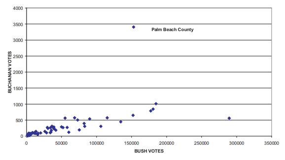
Figure 12.5. Florida presidential vote (all counties).

For example, Figures 12.8 and Figures 12.9 show the regression equations with and without intercepts, respectively, for predicting votes for Buchanan as a function of votes for Nader based on all counties except Palm Beach. We then use these equations to predict the Palm Beach outcome; then we compare our results to the 3407 votes that actually were counted in Palm Beach County as votes for Buchanan.

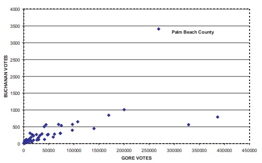
Figure 12.6. Florida presidential votes (all counties).

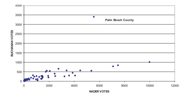
Figure 12.7. Florida presidential votes (all counties).

Since Nader received 5564 votes in Palm Beach County, we derive, using the equation in Figure 12.8, the prediction of Y for Buchanan: Yˆ = 0.1028(5564) + 68.93 = 640.9092. Or, if we use the zero intercept formula, we have Yˆ = 0.1194 (5564) = 664.3416.

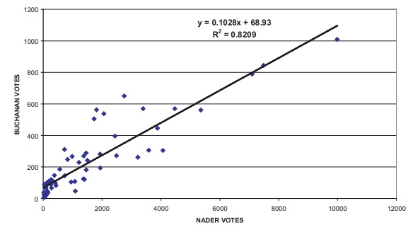
Figure 12.8. Florida presidential vote (Palm Beach county omitted).

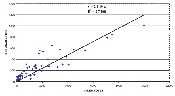
Figure 12.9. Florida presidential vote (Palm Beach county omitted).

Similar predictions for the votes for Buchanan using the votes for Bush as the covariate X give the equations Yˆ = 0.0035 X + 65.51 = 600.471 and Yˆ = 0.004 X = 611.384 (zero intercept formula), since Bush reaped 152,846 votes in Palm Beach County. Votes for Gore also could be used to predict the votes for Buchanan, although the correlation is lower (r = 0.7940 for the equation with intercept, and r = 0.6704 for the equation without the intercept).

Using the votes for Gore, the regression equations are Yˆ = 0.0025 X + 109.24 and Yˆ = 0.0032 X, respectively, for the fit with and without the intercept. Gore’s 268,945 votes in Palm Beach County lead to predictions of 781.6025 and 1075.78 using the intercept and nonintercept equations, respectively.

In all cases, the predictions of votes for Buchanan ranged from around 600 votes to approximately 1076 votes—far less than the 3407 votes that Buchanan actually received. This discrepancy between the number of predicted and actual votes leads to a very plausible argument that at least 2000 of the votes awarded to Buchanan could have been intended for Gore.

An increase in the number of votes for Gore would eliminate the outlier with re-spect to the number of votes cast for Buchanan that were detected for Palm Beach County. This hypothetical increase would be responsive to the complaints of many voters who said they were confused by the butterfly ballot. A study of the ballot shows that the punch hole for Buchanan could be confused with Gore’s but not with that of any other candidate. A better prediction of the vote for Buchanan could be obtained by multiple regression. We will review the data again in Section 12.9.

The undo influence of outliers on regression equations is one of the problems that can be resolved by using robust regression techniques. Many texts on regres-sion models are available that cover robust regression and/or the regression diag-nostics that can be used to determine when the assumptions for least squares regres-sion do not apply. We will not go into the details of these topics; however, in Section 12.12 (Additional Reading), we provide the interested reader with several good texts. These texts include Chatterjee and Hadi (1988); Chatterjee, Price, and Hadi (1999); Ryan (1997); Montgomery, and Peck (1992); Myers (1990); Draper, and Smith (1998); Cook (1998); Belsley, Kuh, and Welsch (1980); Rousseeuw and Leroy (1987); Bloomfield and Steiger (1983); Staudte and Sheather (1990); Cook and Weisberg (1982); and Weisberg (1985).

Some of the aforementioned texts cover diagnostic statistics that are useful for detecting multicollinearity (a problem that occurs when two or more predictor vari-ables in the regression equation have a strong linear interrelationship). Of course, multicollinearity is not a problem when one deals only with a single predictor. When relationships among independent and dependent variables seem to be nonlin-ear, transformation methods sometimes are employed. For these methods, the least squares regression model is fitted to the data after the transformation [see Atkinson (1985) or Carroll and Ruppert (1988)].

As is true of regression equations, outliers can adversely affect estimates of the correlation coefficient. Nonparametric alternatives to the Pearson product moment correlation exist and can be used in such instances. One such alternative, called Spearman’s rho, is covered in Section 14.7.