Coefficient of Variation (CV) and Coefficient of Dispersion (CD)

COEFFICIENT OF VARIATION (CV) AND COEFFICIENT OF DISPERSION (CD)

Useful and meaningful only for variables that take on positive values, the coefficient of variation is defined as the ratio of the standard deviation to the absolute value of the mean. The coefficient of variation is well defined for any variable (includ-ing a variable that can be negative) that has a nonzero mean.

Let θ and V symbolize the coefficient of variation in the population and sample, respectively. Refer to Formulas 4.13a and 4.13b for calculating θ and V.

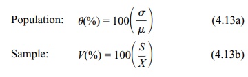
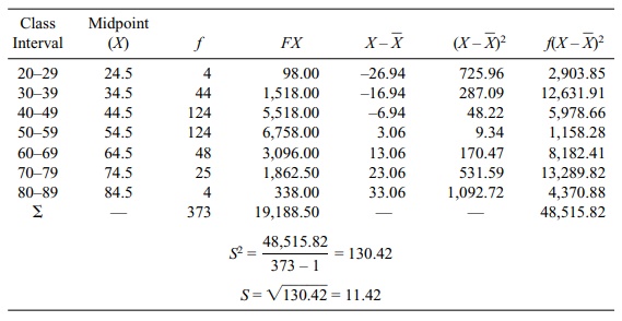
TABLE 4.8. Ages of Patients Diagnosed with Multiple Sclerosis: Sample Variance and Standard Deviation Calculations Using the Formulae for Grouped Data

Usually represented as a percentage, sometimes θ is thought of as a measure of relative dispersion. A variable with a population standard deviation of σ and a mean μ > 0 has a coefficient of variation θ = 100(σ/μ)%.

Given a data set with a sample mean  > 0 and standard deviation S, the sample coefficient of variation is V = 100(S/)%. The term V is the obvious sample analog to the population coefficient of variation.

The original purpose of the coefficient of variation was to make comparisons be-tween different distributions. For instance, if we want to see whether the distribu-tion of the length of the tails of mice is similar to the distribution of the length of elephants’ tails, we could not meaningfully compare their actual standard deviations. In comparison to the standard deviation of the tails of mice, the standard devi-ation of elephants’ tails would be larger simply because of the much larger mea-surement scale being used. However, these very differently sized animals might very well have similar coefficients of variation with respect to their tail lengths.

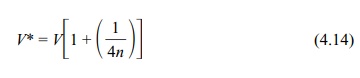
Another estimator, V*, the coefficient of variation biased adjusted estimate, is often used for the sample estimate of the coefficient of variation because it has less bias in estimating θ. V* = V{1 + (1/[4n])}, where n is the sample size. So V* in-creases V by a factor of 1/(4n) or adds V/(4n) to the estimate of V. Formula 4.14 shows the formula for V*:

This estimate and further discussion of the coefficient of variation can be found in Sokal and Rohlf (1981).

Formulas 4.15a and 4.15b present the formula for the coefficient of dispersion (CD):

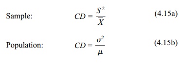
Similar to V, CD is the ratio of the variance to the mean. If we think of V as a ratio rather than a percentage, we see that CD is just V². The coefficient of dispersion is related to the Poisson distribution, which we will explain later in the text. Often, the Poisson distribution is a good model for representing the number of events (e.g., traf-fic accidents in Los Angeles) that occur in a given time interval. The Poisson distrib-ution, which can take on the value zero or any positive value, has the property that its mean is always equal to its variance. So a Poisson random variable has a coefficient of dispersion equal to 1. The CD is the sample estimate of the coefficient of disper-sion. Often, we are interested in count data. You will see many applications of count data when we come to the analysis of survival times in Chapter 15.

We may want to know whether the Poisson distribution is a reasonable model for our data. One way to ascertain the fit of the data to the Poisson distribution is to ex-amine the CD. If we have sufficient data, the CD will provide a good estimate of the population coefficient of dispersion. If the Poisson model is reasonable, the estimat-ed CD should be close to 1. If the CD is much less than 1, then the counting process is said to be underdispersed (meaning that the CD has less variance relative to the mean than a Poisson counting process). On the other hand, a counting process with a value of CD that is much greater than 1 indicates overdispersion (the opposite of underdispersion).

Overdispersion occurs commonly as a counting process that provides a mixture of two or more different Poisson counting processes. These so-called compound Poisson processes occur frequently in nature and also in some manmade events. A hypothetical example relates to the time intervals between motor vehicle accidents in a specific community during a particular year. The data for the time intervals be-tween motor vehicle accidents might fit well to a Poisson process. However, the data aggregate information for all ages, e.g., young people (18–25 years of age), mature adults (25–65 years of age), and the elderly (above 65 years of age). The motor vehicle accident rate is likely to be higher for the inexperienced young peo-ple than for the mature adults. Also, the elderly, because of slower reflexes and poorer vision, are likely to have a higher accident rate than the mature adults. The motor vehicle accident data for the combined population of drivers represents an accumulation of three different Poisson processes (corresponding to three different age groups) and, hence, an overdispersed process.

A key assumption of linear models is that the variance of the response variable Y remains constant as predictor variables change. Miller (1986) points out that a prob-lem with using linear models is that the variance of a response variable often does not remain constant but changes as a function of a predictor variable.

One remedy for response variables that have changing variance when predictor variables change is to use variance-stabilizing transformations. Such transforma-tions produce a variable that has variance that does not change as the mean changes. The mean of the response variable will change in experiments in which the predictor variables are allowed to change; the mean of the response changes because it is affected by these predictors. You will appreciate these notions more fully when we cover correlation and simple linear regression in Chapter 12.

Miller (1986), p. 59, using what is known as the delta method, shows that a log transformation stabilizes the variance when the coefficient of variation for the response remains constant as its mean changes. Similarly, he shows that a square root transformation stabilizes the variance if the coefficient of dispersion for the response remains constant as the mean changes. Miller’s book is advanced and re-quires some familiarity with calculus.

Transformations can be used as tools to achieve statistical assumptions needed for certain types of parametric analyses. The delta method is an approximation technique based on terms in a Taylor series (polynomial approximations to functions). Although understanding a Taylor series requires a first year calculus course, it is sufficient to know that the coefficient of dispersion and the coefficient of variation have statistical properties that make them useful in some analyses.

Because Poisson variables have a constant coefficient of dispersion of 1, the square root transformation will stabilize the variance for them. This fact can be very useful for some practical applications.